🔎大家好,我是Sonhhxg_柒,希望你看完之后,能对你有所帮助,不足请指正!共同学习交流🔎
📝个人主页-Sonhhxg_柒的博客_CSDN博客 📃
🎁欢迎各位→点赞👍 + 收藏⭐️ + 留言📝
📣系列专栏 - 机器学习【ML】 自然语言处理【NLP】 深度学习【DL】
🖍foreword
✔说明⇢本人讲解主要包括Python、机器学习(ML)、深度学习(DL)、自然语言处理(NLP)等内容。
如果你对这个系列感兴趣的话,可以关注订阅哟👋
文章目录
数据探索
处理降雨预测的类不平衡
归因与转化
降雨预测的特征选择
用不同的模型训练降雨预测模型
为所有模型绘制决策区域
降雨预测模型比较
降雨预报是对人类社会有重大影响的困难和不确定性任务之一。及时准确的预测可以主动帮助减少人员和经济损失。这项研究提出了一组实验,涉及使用常见的机器学习技术来创建模型,这些模型可以根据澳大利亚主要城市当天的天气数据预测明天是否会下雨。
我一直喜欢了解气象学家在进行天气预报之前考虑的参数,所以我发现数据集很有趣。然而,从专家的角度来看,这个数据集相当简单。在本文的最后,您将了解到:
- 1.如何为不平衡的数据集进行平衡
- 2.如何对分类变量进行标签编码
- 3.如何使用像 MICE 这样复杂的插补
- 4.如何检测异常值并将其从数据中排除
- 5.filter方法和wrapper方法如何用于特征选择
- 6.如何比较不同流行型号的速度和性能
- 7.哪个指标可以最好地判断不平衡数据集的性能:精度和 F1 分数。
- 让我们通过导入数据开始这个降雨预测任务,你可以从这里下载我在这个任务中使用的数据集:
-
import pandas as pd
from google.colab import files
uploaded = files.upload()
full_data = pd.read_csv('weatherAUS.csv')
full_data.head()
数据探索
我们将首先检查行数和列数。接下来,我们将检查数据集的大小,以确定它是否需要大小压缩。
full_data.shape(142193, 24)full_data.info()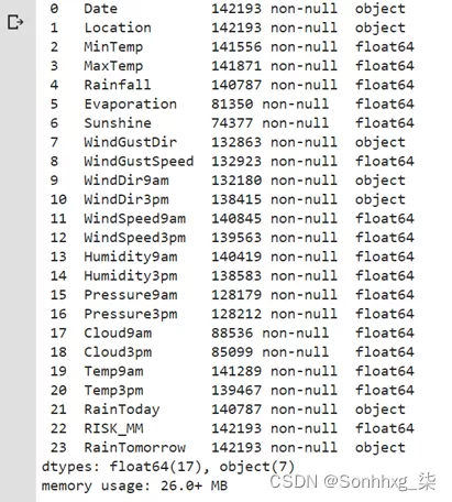
“RainToday”和“RainTomorrow”是对象(是/否)。为了方便起见,我会将它们转换为二进制 (1/0)。
full_data['RainToday'].replace({'No': 0, 'Yes': 1},inplace = True)
full_data['RainTomorrow'].replace({'No': 0, 'Yes': 1},inplace = True)
接下来,我们将检查数据集是不平衡的还是平衡的。如果数据集不平衡,我们需要对大多数数据进行下采样或对少数数据进行过采样以使其平衡。
import matplotlib.pyplot as plt
fig = plt.figure(figsize = (8,5))
full_data.RainTomorrow.value_counts(normalize = True).plot(kind='bar', color= ['skyblue','navy'], alpha = 0.9, rot=0)
plt.title('RainTomorrow Indicator No(0) and Yes(1) in the Imbalanced Dataset')
plt.show()
我们可以观察到“0”和“1”的存在比例几乎是78:22。所以存在阶级不平衡,我们必须处理它。为了对抗类不平衡,我们将在这里使用少数类的过采样。由于数据集的大小非常小,多数类二次抽样在这里没有多大意义。
处理降雨预测的类不平衡
-
from sklearn.utils import resample

no = full_data[full_data.RainTomorrow == 0]
yes = full_data[full_data.RainTomorrow == 1]
yes_oversampled = resample(yes, replace=True, n_samples=len(no), random_state=123)
oversampled = pd.concat([no, yes_oversampled])

fig = plt.figure(figsize = (8,5))
oversampled.RainTomorrow.value_counts(normalize = True).plot(kind='bar', color= ['skyblue','navy'], alpha = 0.9, rot=0)
plt.title('RainTomorrow Indicator No(0) and Yes(1) after Oversampling (Balanced Dataset)')
plt.show()
现在,我将检查数据集中缺失的数据模型:
# Missing Data Pattern in Training Data
import seaborn as sns
sns.heatmap(oversampled.isnull(), cbar=False, cmap='PuBu')
显然,“Evaporation”、“Sunshine”、“Cloud9am”、“Cloud3pm”是缺失率较高的特征。因此,我们将检查这 4 个特征的缺失数据的详细信息。
total = oversampled.isnull().sum().sort_values(ascending=False)
percent = (oversampled.isnull().sum()/oversampled.isnull().count()).sort_values(ascending=False)
missing = pd.concat([total, percent], axis=1, keys=['Total', 'Percent'])
missing.head(4)
Total Percent Sunshine 104831 0.475140 Evaporation 95411 0.432444 Cloud3pm 85614 0.388040 Cloud9am 81339 0.368664我们观察到这 4 个特征的缺失数据不到 50%。因此,我们不会完全拒绝它们,而是会在我们的模型中考虑它们并进行适当的归因。
归因与转化
我们将用众数估算分类列,然后我们将使用标签编码器将它们转换为数字。一旦完整数据框中的所有列都转换为数字列,我们将使用链式方程多重插补 (MICE) 包来插补缺失值。
然后我们将使用四分位间距检测异常值并将它们移除以获得最终的工作数据集。最后,我们将检查不同变量之间的相关性,如果我们发现一对高度相关的变量,我们将丢弃一个而保留另一个。
oversampled.select_dtypes(include=['object']).columnsIndex(['Date', 'Location', 'WindGustDir', 'WindDir9am', 'WindDir3pm'], dtype='object')# Impute categorical var with Mode oversampled['Date'] = oversampled['Date'].fillna(oversampled['Date'].mode()[0]) oversampled['Location'] = oversampled['Location'].fillna(oversampled['Location'].mode()[0]) oversampled['WindGustDir'] = oversampled['WindGustDir'].fillna(oversampled['WindGustDir'].mode()[0]) oversampled['WindDir9am'] = oversampled['WindDir9am'].fillna(oversampled['WindDir9am'].mode()[0]) oversampled['WindDir3pm'] = oversampled['WindDir3pm'].fillna(oversampled['WindDir3pm'].mode()[0])# Convert categorical features to continuous features with Label Encoding from sklearn.preprocessing import LabelEncoder lencoders = {} for col in oversampled.select_dtypes(include=['object']).columns: lencoders[col] = LabelEncoder() oversampled[col] = lencoders[col].fit_transform(oversampled[col])import warnings warnings.filterwarnings("ignore") # Multiple Imputation by Chained Equations from sklearn.experimental import enable_iterative_imputer from sklearn.impute import IterativeImputer MiceImputed = oversampled.copy(deep=True) mice_imputer = IterativeImputer() MiceImputed.iloc[:, :] = mice_imputer.fit_transform(oversampled)因此,数据帧没有“NaN”值。我们现在将从基于四分位数间隔的数据集中检测并消除异常值。
# Detecting outliers with IQR
Q1 = MiceImputed.quantile(0.25)
Q3 = MiceImputed.quantile(0.75)
IQR = Q3 - Q1
print(IQR)
Date 1535.000000 Location 25.000000 MinTemp 9.300000 MaxTemp 10.200000 Rainfall 2.400000 Evaporation 4.119679 Sunshine 5.947404 WindGustDir 9.000000 WindGustSpeed 19.000000 WindDir9am 8.000000 WindDir3pm 8.000000 WindSpeed9am 13.000000 WindSpeed3pm 11.000000 Humidity9am 26.000000 Humidity3pm 30.000000 Pressure9am 8.800000 Pressure3pm 8.800000 Cloud9am 4.000000 Cloud3pm 3.681346 Temp9am 9.300000 Temp3pm 9.800000 RainToday 1.000000 RISK_MM 5.200000 RainTomorrow 1.000000 dtype : float64# Removing outliers from the dataset MiceImputed = MiceImputed[~((MiceImputed < (Q1 - 1.5 * IQR)) |(MiceImputed > (Q3 + 1.5 * IQR))).any(axis=1)] MiceImputed.shape(156852, 24)我们观察到原始数据集的形式为 (87927, 24)。在运行用于移除异常值的代码片段后,数据集现在具有 (86065, 24) 的形式。因此,数据集现在没有 1862 个异常值。我们现在要检查多重共线性,也就是说一个字符是否与另一个字符密切相关。
# Correlation Heatmap
import numpy as np
import matplotlib.pyplot as plt
import seaborn as sns
corr = MiceImputed.corr()
mask = np.triu(np.ones_like(corr, dtype=np.bool))
f, ax = plt.subplots(figsize=(20, 20))
cmap = sns.diverging_palette(250, 25, as_cmap=True)
sns.heatmap(corr, mask=mask, cmap=cmap, vmax=None, center=0,square=True, annot=True, linewidths=.5, cbar_kws={"shrink": .9})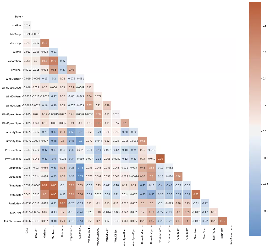
以下特征对彼此具有很强的相关性:
- 1.最高温度和最低温度
- 2.Pressure9h 和 pressure3h
- 3.上午 9 点和下午 3 点
- 4.蒸发和最高温度
- 5.MaxTemp 和 Temp3pm 但在任何情况下相关值都不等于完美的“1”。因此,我们不会删除任何功能
- 4.蒸发和最高温度
- 3.上午 9 点和下午 3 点
- 2.Pressure9h 和 pressure3h
- 1.最高温度和最低温度
-
然而,我们可以通过检查以下配对图来更深入地研究这些高度相关特征之间的成对相关性。每个成对的图都非常清楚地显示了 RainTomorrow 的“是”和“否”集群。它们之间的重叠非常小。
-
sns.pairplot( data=MiceImputed, vars=('MaxTemp','MinTemp','Pressure9am','Pressure3pm', 'Temp9am', 'Temp3pm', 'Evaporation'), hue='RainTomorrow' )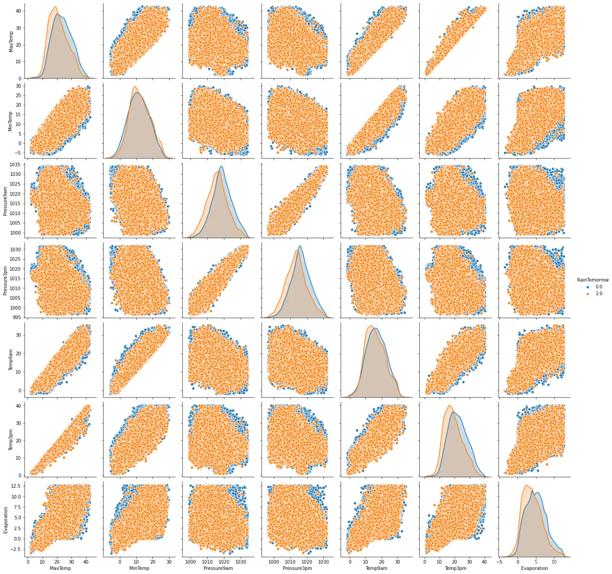
降雨预测的特征选择
我将使用过滤器方法和包装器方法进行特征选择来训练我们的降雨预测模型。
通过过滤方法(卡方值)选择特征:在这样做之前,我们必须先规范化我们的数据。我们使用 MinMaxScaler 而不是 StandardScaler 以避免出现负值。
# Standardizing data
from sklearn import preprocessing
r_scaler = preprocessing.MinMaxScaler()
r_scaler.fit(MiceImputed)
modified_data = pd.DataFrame(r_scaler.transform(MiceImputed), index=MiceImputed.index, columns=MiceImputed.columns)
# Feature Importance using Filter Method (Chi-Square) from sklearn.feature_selection import SelectKBest, chi2 X = modified_data.loc[:,modified_data.columns!='RainTomorrow'] y = modified_data[['RainTomorrow']] selector = SelectKBest(chi2, k=10) selector.fit(X, y) X_new = selector.transform(X) print(X.columns[selector.get_support(indices=True)])Index(['Sunshine', 'Humidity9am', 'Humidity3pm', 'Pressure9am', 'Pressure3pm', 'Cloud9am', 'Cloud3pm', 'Temp3pm', 'RainToday', 'RISK_MM'], dtype='object')我们可以观察到“Sunshine”、“Humidity9am”、“Humidity3pm”、“Pressure9am”、“Pressure3pm”与其他特征相比具有更高的重要性。
通过包装方法(随机森林)选择特征:
from sklearn.feature_selection import SelectFromModel
from sklearn.ensemble import RandomForestClassifier as rf

X = MiceImputed.drop('RainTomorrow', axis=1)
y = MiceImputed['RainTomorrow']
selector = SelectFromModel(rf(n_estimators=100, random_state=0))
selector.fit(X, y)
support = selector.get_support()
features = X.loc[:,support].columns.tolist()
print(features)
print(rf(n_estimators=100, random_state=0).fit(X,y).feature_importances_)
['Sunshine', 'Cloud3pm', 'RISK_MM'] [0.00205993 0.00215407 0.00259089 0.00367568 0.0102656 0.00252838 0.05894157 0.00143001 0.00797518 0.00177178 0.00167654 0.0014278 0.00187743 0.00760691 0.03091966 0.00830365 0.01193018 0.02113544 0.04962418 0.00270103 0.00513723 0.00352198 0.76074491]用不同的模型训练降雨预测模型
我们将数据集分为训练集(75%)和测试集(25%)来训练降雨预测模型。为了获得最佳结果,我们将标准化 X_train 和 X_test 数据:
features = MiceImputed[['Location', 'MinTemp', 'MaxTemp', 'Rainfall', 'Evaporation', 'Sunshine', 'WindGustDir',
                       'WindGustSpeed', 'WindDir9am', 'WindDir3pm', 'WindSpeed9am', 'WindSpeed3pm', 'Humidity9am',
                       'Humidity3pm', 'Pressure9am', 'Pressure3pm', 'Cloud9am', 'Cloud3pm', 'Temp9am', 'Temp3pm',
                       'RainToday']]
target = MiceImputed['RainTomorrow']

# Split into test and train
from sklearn.model_selection import train_test_split
X_train, X_test, y_train, y_test = train_test_split(features, target, test_size=0.25, random_state=12345)

# Normalize Features
from sklearn.preprocessing import StandardScaler
scaler = StandardScaler()
X_train = scaler.fit_transform(X_train)
X_test = scaler.fit_transform(X_test)
def plot_roc_cur(fper, tper): plt.plot(fper, tper, color='orange', label='ROC') plt.plot([0, 1], [0, 1], color='darkblue', linestyle='--') plt.xlabel('False Positive Rate') plt.ylabel('True Positive Rate') plt.title('Receiver Operating Characteristic (ROC) Curve') plt.legend() plt.show()import time from sklearn.metrics import accuracy_score, roc_auc_score, cohen_kappa_score, plot_confusion_matrix, roc_curve, classification_report def run_model(model, X_train, y_train, X_test, y_test, verbose=True): t0=time.time() if verbose == False: model.fit(X_train,y_train, verbose=0) else: model.fit(X_train,y_train) y_pred = model.predict(X_test) accuracy = accuracy_score(y_test, y_pred) roc_auc = roc_auc_score(y_test, y_pred) coh_kap = cohen_kappa_score(y_test, y_pred) time_taken = time.time()-t0 print("Accuracy = {}".format(accuracy)) print("ROC Area under Curve = {}".format(roc_auc)) print("Cohen's Kappa = {}".format(coh_kap)) print("Time taken = {}".format(time_taken)) print(classification_report(y_test,y_pred,digits=5)) probs = model.predict_proba(X_test) probs = probs[:, 1] fper, tper, thresholds = roc_curve(y_test, probs) plot_roc_cur(fper, tper) plot_confusion_matrix(model, X_test, y_test,cmap=plt.cm.Blues, normalize = 'all') return model, accuracy, roc_auc, coh_kap, time_taken# Logistic Regression from sklearn.linear_model import LogisticRegression params_lr = {'penalty': 'l1', 'solver':'liblinear'} model_lr = LogisticRegression(**params_lr) model_lr, accuracy_lr, roc_auc_lr, coh_kap_lr, tt_lr = run_model(model_lr, X_train, y_train, X_test, y_test) # Decision Tree from sklearn.tree import DecisionTreeClassifier params_dt = {'max_depth': 16, 'max_features': "sqrt"} model_dt = DecisionTreeClassifier(**params_dt) model_dt, accuracy_dt, roc_auc_dt, coh_kap_dt, tt_dt = run_model(model_dt, X_train, y_train, X_test, y_test) # Neural Network from sklearn.neural_network import MLPClassifier params_nn = {'hidden_layer_sizes': (30,30,30), 'activation': 'logistic', 'solver': 'lbfgs', 'max_iter': 500} model_nn = MLPClassifier(**params_nn) model_nn, accuracy_nn, roc_auc_nn, coh_kap_nn, tt_nn = run_model(model_nn, X_train, y_train, X_test, y_test) # Random Forest from sklearn.ensemble import RandomForestClassifier params_rf = {'max_depth': 16, 'min_samples_leaf': 1, 'min_samples_split': 2, 'n_estimators': 100, 'random_state': 12345} model_rf = RandomForestClassifier(**params_rf) model_rf, accuracy_rf, roc_auc_rf, coh_kap_rf, tt_rf = run_model(model_rf, X_train, y_train, X_test, y_test) # Light GBM import lightgbm as lgb params_lgb ={'colsample_bytree': 0.95, 'max_depth': 16, 'min_split_gain': 0.1, 'n_estimators': 200, 'num_leaves': 50, 'reg_alpha': 1.2, 'reg_lambda': 1.2, 'subsample': 0.95, 'subsample_freq': 20} model_lgb = lgb.LGBMClassifier(**params_lgb) model_lgb, accuracy_lgb, roc_auc_lgb, coh_kap_lgb, tt_lgb = run_model(model_lgb, X_train, y_train, X_test, y_test) # Catboost !pip install catboost import catboost as cb params_cb ={'iterations': 50, 'max_depth': 16} model_cb = cb.CatBoostClassifier(**params_cb) model_cb, accuracy_cb, roc_auc_cb, coh_kap_cb, tt_cb = run_model(model_cb, X_train, y_train, X_test, y_test, verbose=False) # XGBoost import xgboost as xgb params_xgb ={'n_estimators': 500, 'max_depth': 16} model_xgb = xgb.XGBClassifier(**params_xgb) model_xgb, accuracy_xgb, roc_auc_xgb, coh_kap_xgb, tt_xgb = run_model(model_xgb, X_train, y_train, X_test, y_test)为所有模型绘制决策区域
import numpy as np
import matplotlib.pyplot as plt
import matplotlib.gridspec as gridspec
import itertools
from sklearn.linear_model import LogisticRegression
from sklearn.tree import DecisionTreeClassifier
from sklearn.neural_network import MLPClassifier
from sklearn.ensemble import RandomForestClassifier
import lightgbm as lgb
import catboost as cb
import xgboost as xgb
from mlxtend.classifier import EnsembleVoteClassifier
from mlxtend.plotting import plot_decision_regions

value = 1.80
width = 0.90

clf1 = LogisticRegression(random_state=12345)
clf2 = DecisionTreeClassifier(random_state=12345)
clf3 = MLPClassifier(random_state=12345, verbose = 0)
clf4 = RandomForestClassifier(random_state=12345)
clf5 = lgb.LGBMClassifier(random_state=12345, verbose = 0)
clf6 = cb.CatBoostClassifier(random_state=12345, verbose = 0)
clf7 = xgb.XGBClassifier(random_state=12345)
eclf = EnsembleVoteClassifier(clfs=[clf4, clf5, clf6, clf7], weights=[1, 1, 1, 1], voting='soft')

X_list = MiceImputed[["Sunshine", "Humidity9am", "Cloud3pm"]] #took only really important features
X = np.asarray(X_list, dtype=np.float32)
y_list = MiceImputed["RainTomorrow"]
y = np.asarray(y_list, dtype=np.int32)

# Plotting Decision Regions
gs = gridspec.GridSpec(3,3)
fig = plt.figure(figsize=(18, 14))

labels = ['Logistic Regression',
          'Decision Tree',
          'Neural Network',
          'Random Forest',
          'LightGBM',
          'CatBoost',
          'XGBoost',
          'Ensemble']

for clf, lab, grd in zip([clf1, clf2, clf3, clf4, clf5, clf6, clf7, eclf],
                         labels,
                         itertools.product([0, 1, 2],
                         repeat=2)):
    clf.fit(X, y)
    ax = plt.subplot(gs[grd[0], grd[1]])
    fig = plot_decision_regions(X=X, y=y, clf=clf,
                                filler_feature_values={2: value},
                                filler_feature_ranges={2: width},
                                legend=2)
    plt.title(lab)

plt.show()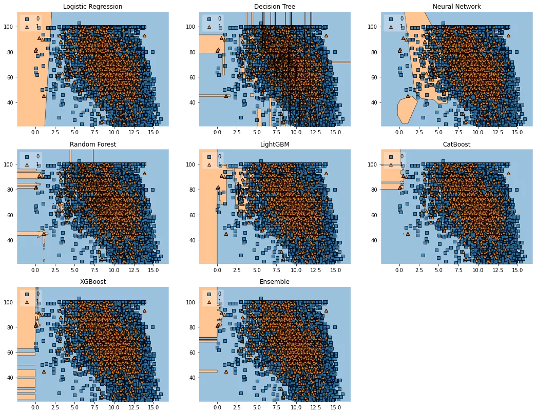
我们可以观察到不同模型的类别限制的差异,包括集合模型(该图仅考虑训练数据)。与所有其他模型相比,CatBoost 具有明显的区域边界。然而,与其他模型相比,XGBoost 和随机森林模型的错误分类数据点数量也少得多。
降雨预测模型比较
现在我们需要根据 Precision Score、ROC_AUC、Cohen's Kappa 和 Total Run Time 来决定哪个模型表现最好。这里要提到的一点是:我们本可以将 F1-Score 视为判断模型性能而不是准确性的更好指标,但我们已经将不平衡数据集转换为平衡数据集,因此将准确性视为决定最佳模型的指标在这种情况下是合理的。
为了做出更好的决定,我们选择了“Cohen's Kappa”,这实际上是一个理想的选择,作为在数据集不平衡的情况下决定最佳模型的指标。让我们检查一下哪个模型在哪个方面运行良好:
accuracy_scores = [accuracy_lr, accuracy_dt, accuracy_nn, accuracy_rf, accuracy_lgb, accuracy_cb, accuracy_xgb]
roc_auc_scores = [roc_auc_lr, roc_auc_dt, roc_auc_nn, roc_auc_rf, roc_auc_lgb, roc_auc_cb, roc_auc_xgb]
coh_kap_scores = [coh_kap_lr, coh_kap_dt, coh_kap_nn, coh_kap_rf, coh_kap_lgb, coh_kap_cb, coh_kap_xgb]
tt = [tt_lr, tt_dt, tt_nn, tt_rf, tt_lgb, tt_cb, tt_xgb]

model_data = {'Model': ['Logistic Regression','Decision Tree','Neural Network','Random Forest','LightGBM','Catboost','XGBoost'],
              'Accuracy': accuracy_scores,
              'ROC_AUC': roc_auc_scores,
              'Cohen_Kappa': coh_kap_scores,
              'Time taken': tt}
data = pd.DataFrame(model_data)

fig, ax1 = plt.subplots(figsize=(12,10))
ax1.set_title('Model Comparison: Accuracy and Time taken for execution', fontsize=13)
color = 'tab:green'
ax1.set_xlabel('Model', fontsize=13)
ax1.set_ylabel('Time taken', fontsize=13, color=color)
ax2 = sns.barplot(x='Model', y='Time taken', data = data, palette='summer')
ax1.tick_params(axis='y')
ax2 = ax1.twinx()
color = 'tab:red'
ax2.set_ylabel('Accuracy', fontsize=13, color=color)
ax2 = sns.lineplot(x='Model', y='Accuracy', data = data, sort=False, color=color)
ax2.tick_params(axis='y', color=color)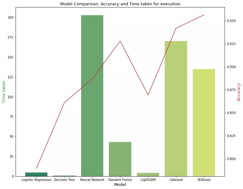
fig, ax3 = plt.subplots(figsize=(12,10))
ax3.set_title('Model Comparison: Area under ROC and Cohens Kappa', fontsize=13)
color = 'tab:blue'
ax3.set_xlabel('Model', fontsize=13)
ax3.set_ylabel('ROC_AUC', fontsize=13, color=color)
ax4 = sns.barplot(x='Model', y='ROC_AUC', data = data, palette='winter')
ax3.tick_params(axis='y')
ax4 = ax3.twinx()
color = 'tab:red'
ax4.set_ylabel('Cohen_Kappa', fontsize=13, color=color)
ax4 = sns.lineplot(x='Model', y='Cohen_Kappa', data = data, sort=False, color=color)
ax4.tick_params(axis='y', color=color)
plt.show()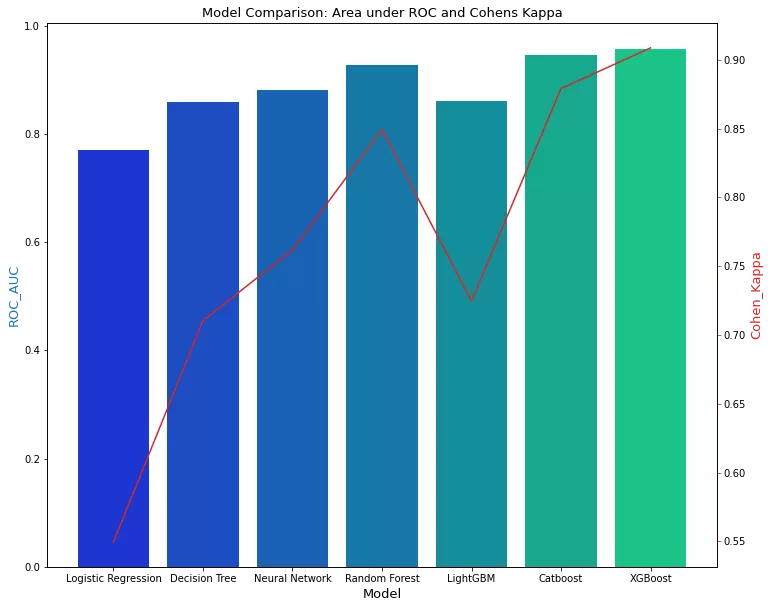
我们可以观察到 XGBoost、CatBoost 和随机森林与其他模型相比表现更好。然而,如果速度是一个重要的考虑因素,我们可以坚持使用随机森林而不是 XGBoost 或 CatBoost。
我希望您喜欢这篇关于我们如何创建和比较不同降雨预测模型的文章。
- 6.如何比较不同流行型号的速度和性能
- 5.filter方法和wrapper方法如何用于特征选择
- 4.如何检测异常值并将其从数据中排除
- 3.如何使用像 MICE 这样复杂的插补
- 2.如何对分类变量进行标签编码


![[Linux]多线程的同步和互斥(线程池 | 单例模式 | 其他常见的锁 | 读者写者问题)](https://img-blog.csdnimg.cn/7caa02ae52c34f64a4d362f55c2b8006.png)