01_introduction_to_diffusers

🤗 Diffusers 介绍

来源：https://github.com/huggingface/diffusion-models-class/blob/main/unit1/01_introduction_to_diffusers.ipynb

预备知识

在进入 Notebook 之前，你需要:

📖 阅读第一单元的材料
🤗 在 Hugging Face Hub 上创建一个账户。你可以在这里完成注册: https://huggingface.co/join

步骤 1: 设置

运行以下单元以安装 diffusers 库以及一些其他要求：

%pip install -qq -U diffusers datasets transformers accelerate ftfy pyarrow

接下来，请前往 https://huggingface.co/settings/tokens 创建具有写权限的访问令牌：

你可以使用命令行来通过此令牌登录 (huggingface-cli login) 或者运行以下单元来登录：

from huggingface_hub import notebook_login

notebook_login()

VBox(children=(HTML(value='<center> <img\nsrc=https://huggingface.co/front/assets/huggingface_logo-noborder.sv…

然后你需要安装 Git LFS 来上传模型检查点：

%%capture
!sudo apt -qq install git-lfs
!git config --global credential.helper store

最后，让我们导入将要使用的库，并定义一些方便函数，稍后我们将会在 Notebook 中使用这些函数：

import numpy as np
import torch
import torch.nn.functional as F
from matplotlib import pyplot as plt
from PIL import Image


def show_images(x):
    """Given a batch of images x, make a grid and convert to PIL"""
    x = x * 0.5 + 0.5  # Map from (-1, 1) back to (0, 1)
    grid = torchvision.utils.make_grid(x)
    grid_im = grid.detach().cpu().permute(1, 2, 0).clip(0, 1) * 255
    grid_im = Image.fromarray(np.array(grid_im).astype(np.uint8))
    return grid_im


def make_grid(images, size=64):
    """Given a list of PIL images, stack them together into a line for easy viewing"""
    output_im = Image.new("RGB", (size * len(images), size))
    for i, im in enumerate(images):
        output_im.paste(im.resize((size, size)), (i * size, 0))
    return output_im


# Mac users may need device = 'mps' (untested)
device = torch.device("cuda" if torch.cuda.is_available() else "cpu")

好了，我们都准备好了！

Dreambooth：即将到来的巅峰

如果你在过去几个月里看过人工智能相关的社交媒体，你就会听说过 Stable Diffusion 模型。这是一个强大的文本条件隐式扩散模型（别担心，我们将会学习这些概念）。但它有一个缺点：它不知道你或我长什么样，除非我们足够出名以至于互联网上发布我们的照片。

Dreambooth 允许我们创建自己的模型变体，并对特定的面部、对象或样式有一些额外的了解。Corridor Crew 制作了一段出色的视频，用一致的任务形象来讲故事，这是一个很好的说明了这种技术的能力的例子：

from IPython.display import YouTubeVideo

YouTubeVideo("W4Mcuh38wyM")

这是一个使用了这个模型的例子。该模型的训练使用了 5 张著名的儿童玩具 "Mr Potato Head"的照片。

首先，让我们来加载这个管道。这些代码会自动从 Hub 下载模型权重等需要的文件。由于这个只有一行的 demo 需要下载数 GB 的数据，因此你可以跳过此单元格，只需欣赏样例输出即可！

from diffusers import StableDiffusionPipeline

# Check out https://huggingface.co/sd-dreambooth-library for loads of models from the community
model_id = "sd-dreambooth-library/mr-potato-head"

# Load the pipeline
pipe = StableDiffusionPipeline.from_pretrained(model_id, torch_dtype=torch.float16).to(
    device
)

管道加载完成后，我们可以使用以下命令生成图像：

prompt = "an abstract oil painting of sks mr potato head by picasso"
image = pipe(prompt, num_inference_steps=50, guidance_scale=7.5).images[0]
image

0%|          | 0/51 [00:00<?, ?it/s]

在这里插入图片描述

外链图片转存失败,源站可能有防盗链机制,建议将图片保存下来直接上传

练习: 你可以使用不同的提示 (prompt) 自行尝试。在这个 demo 中，sks是一个新概念的唯一标识符 (UID) - 那么如果把它留空的话会发生什么事呢？你还可以尝试改变num_inference_steps和guidance_scale。这两个参数分别代表了采样步骤的数量（试试最多可以设为多低？）和模型将花多大的努力来尝试匹配提示。

这条神奇的管道里有很多事情！课程结束时，你将知道这一切是如何运作的。现在，让我们看看如何从头开始训练扩散模型。

MVP (最简可实行管道)

🤗 Diffusers 的核心 API 被分为三个主要部分:

管道: 从高层出发设计的多种类函数，旨在以易部署的方式，能够做到快速通过主流预训练好的扩散模型来生成样本。
模型: 训练新的扩散模型时用到的主流网络架构，e.g. UNet.
管理器 (or 调度器): 在推理中使用多种不同的技巧来从噪声中生成图像，同时也可以生成在训练中所需的带噪图像。

管道对于末端使用者来说已经非常棒，但你既然已经参加了这门课程，我们就索性认为你想了解更多其中的奥秘！在此篇笔记结束之后，我们会来构建属于你自己，能够生成小蝴蝶图片的管道。下面这里会是最终的结果：

from diffusers import DDPMPipeline

# Load the butterfly pipeline
butterfly_pipeline = DDPMPipeline.from_pretrained(
    "johnowhitaker/ddpm-butterflies-32px"
).to(device)

# Create 8 images
images = butterfly_pipeline(batch_size=8).images

# View the result
make_grid(images)

diffusion_pytorch_model.safetensors not found



Loading pipeline components...:   0%|          | 0/2 [00:00<?, ?it/s]



  0%|          | 0/1000 [00:00<?, ?it/s]

外链图片转存失败,源站可能有防盗链机制,建议将图片保存下来直接上传

也许这看起来并不如 DreamBooth 所展示的样例那样惊艳，但要知道我们在训练这些图画时只用了不到训练稳定扩散模型用到数据的 0.0001%。说到模型训练，从引入介绍直到本单元，训练一个扩散模型的流程看起来像是这样：

从训练集中加载一些图像
加入噪声，从不同程度上
把带了不同版本噪声的数据送进模型
评估模型在对这些数据做增强去噪时的表现
使用这个信息来更新模型权重，然后重复此步骤

步骤 2：下载一个训练数据集

在这个例子中，我们会用到一个来自 Hugging Face Hub 的图像集。具体来说，是个 1000 张蝴蝶图像收藏集. 这是个非常小的数据集，我们这里也同时包含了已被注释的内容指向一些规模更大的选择。如果你想使用你自己的图像收藏，你也可以使用这里被注释掉的示例代码，从一个指定的文件夹来装载图片。

import torchvision
from datasets import load_dataset
from torchvision import transforms

dataset = load_dataset("huggan/smithsonian_butterflies_subset", split="train")

# Or load images from a local folder
# dataset = load_dataset("imagefolder", data_dir="path/to/folder")

# We'll train on 32-pixel square images, but you can try larger sizes too
image_size = 32
# You can lower your batch size if you're running out of GPU memory
batch_size = 64

# Define data augmentations
preprocess = transforms.Compose(
    [
        transforms.Resize((image_size, image_size)),  # Resize
        transforms.RandomHorizontalFlip(),  # Randomly flip (data augmentation)
        transforms.ToTensor(),  # Convert to tensor (0, 1)
        transforms.Normalize([0.5], [0.5]),  # Map to (-1, 1)
    ]
)


def transform(examples):
    images = [preprocess(image.convert("RGB")) for image in examples["image"]]
    return {"images": images}


dataset.set_transform(transform)

# Create a dataloader from the dataset to serve up the transformed images in batches
train_dataloader = torch.utils.data.DataLoader(
    dataset, batch_size=batch_size, shuffle=True
)

Repo card metadata block was not found. Setting CardData to empty.

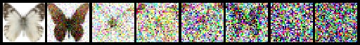
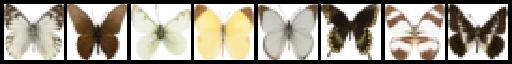
我们可以从中取出一批图像数据来看一看他们是什么样子:

xb = next(iter(train_dataloader))["images"].to(device)[:8]
print("X shape:", xb.shape)
show_images(xb).resize((8 * 64, 64), resample=Image.NEAREST)

X shape: torch.Size([8, 3, 32, 32])

在这里插入图片描述

我们在此篇笔记中使用一个只有 32 像素的小图片集来保证训练时长是可控的。

步骤 3：定义管理器

我们的训练计划是，取出这些输入图片然后对它们增添噪声，在这之后把带噪的图片送入模型。在推理阶段，我们将用模型的预测值来不断迭代去除这些噪点。在diffusers中，这两个步骤都是由 管理器（调度器） 来处理的。

噪声管理器决定在不同的迭代周期时分别加入多少噪声。我们可以这样创建一个管理器，是取自于训练并能取样 ‘DDPM’ 的默认配置。 (基于此篇论文 “Denoising Diffusion Probabalistic Models”:

from diffusers import DDPMScheduler

noise_scheduler = DDPMScheduler(num_train_timesteps=1000)

DDPM 论文这样来描述一个损坏过程，为每一个 ’ 迭代周期 '(timestep) 增添一点少量的噪声。设在某个迭代周期有 $x_{t-1}$ , 我们可以得到它的下一个版本 $x_t$ （比之前更多一点点噪声）:

$(\mathbf {x}_t \vert \mathbf {x}_{t-1}) = \mathcal {N}(\mathbf {x}_t; \sqrt {1 - \beta_t} \mathbf {x}_{t-1}, \beta_t\mathbf {I}) \quad q (\mathbf {x}_{1:T} \vert \mathbf {x}_0) = \prod^T_{t=1} q (\mathbf {x}_t \vert \mathbf {x}_{t-1})$

这就是说，我们取 $x_{t-1}$ , 给他一个 $\sqrt {1 - \beta_t}$ 的系数，然后加上带有 $\beta_t$ 系数的噪声。这里 $\beta$ 是根据一些管理器来为每一个 t 设定的，来决定每一个迭代周期中添加多少噪声。现在，我们不想把这个推演进行 500 次来得到 $x_{500}$ ，所以我们用另一个公式来根据给出的 $x_0$ 计算得到任意 t 时刻的 $x_t$ :

$\begin {aligned} q (\mathbf {x}_t \vert \mathbf {x}_0) &= \mathcal {N}(\mathbf {x}_t; \sqrt {\bar {\alpha}_t} \mathbf {x}_0, {(1 - \bar {\alpha}_t)} \mathbf {I}) \end {aligned}$ where $\bar {\alpha}_t = \prod_{i=1}^T \alpha_i$ and $\alpha_i = 1-\beta_i$

数学符号看起来总是很可怕！好在有管理器来为我们完成这些运算。我们可以画出 $\sqrt {\bar {\alpha}_t}$ (标记为sqrt_alpha_prod) 和 $\sqrt {(1 - \bar {\alpha}_t)}$ (标记为sqrt_one_minus_alpha_prod) 来看一下输入 (x) 与噪声是如何在不同迭代周期中量化和叠加的:

plt.plot(noise_scheduler.alphas_cumprod.cpu() ** 0.5, label=r"${\sqrt{\bar{\alpha}_t}}$")
plt.plot((1 - noise_scheduler.alphas_cumprod.cpu()) ** 0.5, label=r"$\sqrt{(1 - \bar{\alpha}_t)}$")
plt.legend(fontsize="x-large");

在这里插入图片描述

练习: 你可以探索一下使用不同的 beta_start 时曲线是如何变化的，beta_end 与 beta_schedule 可以通过以下注释内容来修改:

# One with too little noise added:
noise_scheduler = DDPMScheduler(num_train_timesteps=1000, beta_start=0.001, beta_end=0.004)
# The 'cosine' schedule, which may be better for small image sizes:
noise_scheduler = DDPMScheduler(num_train_timesteps=1000, beta_schedule='squaredcos_cap_v2')

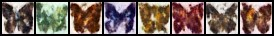
不论你选择了哪一个管理器 (调度器)，我们现在都可以使用noise_scheduler.add_noise功能来添加不同程度的噪声，就像这样：

timesteps = torch.linspace(0, 999, 8).long().to(device)
noise = torch.randn_like(xb)
noisy_xb = noise_scheduler.add_noise(xb, noise, timesteps)
print("Noisy X shape", noisy_xb.shape)
show_images(noisy_xb).resize((8 * 64, 64), resample=Image.NEAREST)

Noisy X shape torch.Size([8, 3, 32, 32])

在这里插入图片描述

再来，在这里探索使用这里不同噪声管理器和预设参数带来的效果。 This video 这个视频很好的解释了一些上述数学运算的细节，同时也是对此类概念的一个很好引入介绍。

步骤 4：定义模型

现在我们来到了核心部分：模型本身。

大多数扩散模型使用的模型结构都是一些 [U-net] 的变形 (https://arxiv.org/abs/1505.04597) 也是我们在这里会用到的结构。

在这里插入图片描述

概括来说:

输入模型中的图片经过几个由 ResNetLayer 构成的层，其中每层都使图片尺寸减半。
之后在经过同样数量的层把图片升采样。
其中还有对特征在相同位置的上、下采样层残差连接模块。

模型一个关键特征既是，输出图片尺寸与输入图片相同，这正是我们这里需要的。

Diffusers 为我们提供了一个易用的UNet2DModel类，用来在 PyTorch 创建所需要的结构。

我们来使用 U-net 为我们生成目标大小的图片吧。
注意这里down_block_types对应下采样模块 (上图中绿色部分), 而up_block_types对应上采样模块 (上图中红色部分):

from diffusers import UNet2DModel

# Create a model
model = UNet2DModel(
    sample_size=image_size,  # the target image resolution
    in_channels=3,  # the number of input channels, 3 for RGB images
    out_channels=3,  # the number of output channels
    layers_per_block=2,  # how many ResNet layers to use per UNet block
    block_out_channels=(64, 128, 128, 256),  # More channels -> more parameters
    down_block_types=(
        "DownBlock2D",  # a regular ResNet downsampling block
        "DownBlock2D",
        "AttnDownBlock2D",  # a ResNet downsampling block with spatial self-attention
        "AttnDownBlock2D",
    ),
    up_block_types=(
        "AttnUpBlock2D",
        "AttnUpBlock2D",  # a ResNet upsampling block with spatial self-attention
        "UpBlock2D",
        "UpBlock2D",  # a regular ResNet upsampling block
    ),
)
model.to(device);

当在处理更高分辨率的输入时，你可能想用更多层的下、上采样模块，让注意力层只聚焦在最低分辨率（最底）层来减少内存消耗。我们在之后会讨论该如何实验来找到最适用与你手头场景的配置方法。

我们可以通过输入一批数据和随机的迭代周期数来看输出是否与输入尺寸相同：

with torch.no_grad():
    model_prediction = model(noisy_xb, timesteps).sample
model_prediction.shape

torch.Size([8, 3, 32, 32])

在下一步中，我们来看如何训练这个模型。

步骤 5：创建训练循环

终于可以训练了！下面这是 PyTorch 中经典的优化迭代循环，在这里一批一批的送入数据然后通过优化器来一步步更新模型参数 - 在这个样例中我们使用学习率为 0.0004 的 AdamW 优化器。

对于每一批的数据，我们要

随机取样几个迭代周期
根据预设为数据加入噪声
把带噪数据送入模型
使用 MSE 作为损失函数来比较目标结果与模型预测结果（在这里是加入噪声的场景）
通过loss.backward ()与optimizer.step ()来更新模型参数

在这个过程中我们记录 Loss 值用来后续的绘图。

NB: 这段代码大概需 10 分钟来运行 - 你也可以跳过以下两块操作直接使用预训练好的模型。供你选择，你可以探索下通过缩小模型层中的通道数会对运行速度有多少提升。

官方扩散模型示例 official diffusers training example 训练了在更高分辨率数据集上的一个更大的模型，这也是一个极为精简训练循环的优秀示例：

# Set the noise scheduler
noise_scheduler = DDPMScheduler(
    num_train_timesteps=1000, beta_schedule="squaredcos_cap_v2"
)

# Training loop
optimizer = torch.optim.AdamW(model.parameters(), lr=4e-4)

losses = []

for epoch in range(30):
    for step, batch in enumerate(train_dataloader):
        clean_images = batch["images"].to(device)
        # Sample noise to add to the images
        noise = torch.randn(clean_images.shape).to(clean_images.device)
        bs = clean_images.shape[0]

        # Sample a random timestep for each image
        timesteps = torch.randint(
            0, noise_scheduler.num_train_timesteps, (bs,), device=clean_images.device
        ).long()

        # Add noise to the clean images according to the noise magnitude at each timestep
        noisy_images = noise_scheduler.add_noise(clean_images, noise, timesteps)

        # Get the model prediction
        noise_pred = model(noisy_images, timesteps, return_dict=False)[0]

        # Calculate the loss
        loss = F.mse_loss(noise_pred, noise)
        loss.backward(loss)
        losses.append(loss.item())

        # Update the model parameters with the optimizer
        optimizer.step()
        optimizer.zero_grad()

    if (epoch + 1) % 5 == 0:
        loss_last_epoch = sum(losses[-len(train_dataloader) :]) / len(train_dataloader)
        print(f"Epoch:{epoch+1}, loss: {loss_last_epoch}")

F:\software\Anaconda\envs\py310\lib\site-packages\diffusers\configuration_utils.py:134: FutureWarning: Accessing config attribute `num_train_timesteps` directly via 'DDPMScheduler' object attribute is deprecated. Please access 'num_train_timesteps' over 'DDPMScheduler's config object instead, e.g. 'scheduler.config.num_train_timesteps'.
  deprecate("direct config name access", "1.0.0", deprecation_message, standard_warn=False)


Epoch:5, loss: 0.15061683766543865
Epoch:10, loss: 0.1153581878170371
Epoch:15, loss: 0.09577085357159376
Epoch:20, loss: 0.09109480120241642
Epoch:25, loss: 0.0887334430590272
Epoch:30, loss: 0.07734946440905333

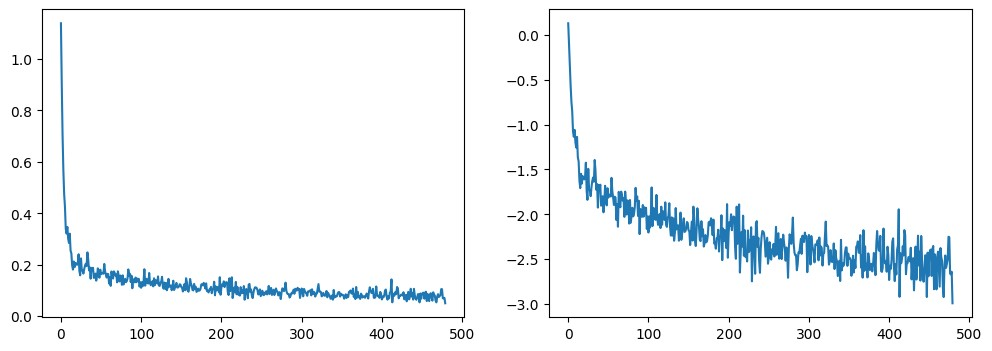
绘制 loss 曲线，我们能看到模型在一开始快速的收敛，接下来以一个较慢的速度持续优化（我们用右边 log 坐标轴的视图可以看的更清楚）：

fig, axs = plt.subplots(1, 2, figsize=(12, 4))
axs[0].plot(losses)
axs[1].plot(np.log(losses))
plt.show()

在这里插入图片描述

你可以选择运行上面的代码，也可以这样通过管道来调用模型：

# Uncomment to instead load the model I trained earlier:
# model = butterfly_pipeline.unet

步骤 6：生成图像

我们怎么从这个模型中得到图像呢？

方法 1：建立一个管道：

from diffusers import DDPMPipeline

image_pipe = DDPMPipeline(unet=model, scheduler=noise_scheduler)

pipeline_output = image_pipe()
pipeline_output.images[0]

  0%|          | 0/1000 [00:00<?, ?it/s]

在这里插入图片描述

我们可以在本地文件夹这样保存一个管道：

image_pipe.save_pretrained("my_pipeline")

检查文件夹的内容：

!ls my_pipeline/

'ls' 不是内部或外部命令，也不是可运行的程序
或批处理文件。

这里scheduler与unet子文件夹中包含了生成图像所需的全部组件。比如，在unet文件中能看到模型参数 (diffusion_pytorch_model.bin) 与描述模型结构的配置文件。

!ls my_pipeline/unet/

'ls' 不是内部或外部命令，也不是可运行的程序
或批处理文件。

以上，这些文件包含了重新建立一个管道的全部内容。你可以手动把它们上传到 hub 来与他人分享你制作的管道，或使用下一节的 API 方法来记载。

方法 2：写一个取样循环

如果你去查看了管道中的 forward 方法，你可以看到在运行image_pipe ()时发生了什么：

# ??image_pipe.forward

从随机噪声开始，遍历管理器的迭代周期来看从最嘈杂直到最微小的噪声变化，基于模型的预测一步步减少一些噪声：

# Random starting point (8 random images):
sample = torch.randn(8, 3, 32, 32).to(device)

for i, t in enumerate(noise_scheduler.timesteps):

    # Get model pred
    with torch.no_grad():
        residual = model(sample, t).sample

    # Update sample with step
    sample = noise_scheduler.step(residual, t, sample).prev_sample

show_images(sample)

在这里插入图片描述

noise_scheduler.step () 函数相应做了 sample（取样）时的数学运算。其实有很多取样的方法 - 在下一个单元我们将看到在已有模型的基础上如何换一个不同的取样器来加速图片生成，也会讲到更多从扩散模型中取样的背后原理。

步骤 7：把你的模型 Push 到 Hub

在上面的例子中我们把管道保存在了本地。把模型 push 到 hub 上，我们会需要建立模型和相应文件的仓库名。我们根据你的选择（模型 ID）来决定仓库的名字（大胆的去替换掉model_name吧；需要包含你的用户名，get_full_repo_name ()会帮你做到）：

from huggingface_hub import get_full_repo_name

model_name = "sd-class-butterflies-32"
hub_model_id = get_full_repo_name(model_name)
hub_model_id

'yuekitty/sd-class-butterflies-32'

然后，在 🤗 Hub 上创建模型仓库并 push 它吧：

from huggingface_hub import HfApi, create_repo

create_repo(hub_model_id)
api = HfApi()
api.upload_folder(
    folder_path="my_pipeline/scheduler", path_in_repo="", repo_id=hub_model_id
)
api.upload_folder(folder_path="my_pipeline/unet", path_in_repo="", repo_id=hub_model_id)
api.upload_file(
    path_or_fileobj="my_pipeline/model_index.json",
    path_in_repo="model_index.json",
    repo_id=hub_model_id,
)

diffusion_pytorch_model.safetensors:   0%|          | 0.00/74.2M [00:00<?, ?B/s]





'https://huggingface.co/yuekitty/sd-class-butterflies-32/blob/main/model_index.json'

hub_model_id

'yuekitty/sd-class-butterflies-32'

最后一件事是创建一个超棒的模型卡，如此，我们的蝴蝶生成器可以轻松的在 Hub 上被找到（请在描述中随意发挥！）：

# encoding:utf-8
from huggingface_hub import ModelCard

content = f"""
---
license: mit
tags:
- pytorch
- diffusers
- unconditional-image-generation
- diffusion-models-class
---

# Model Card for Unit 1 of the [Diffusion Models Class ](https://github.com/huggingface/diffusion-models-class)

This model is a diffusion model for unconditional image generation of cute Butterfly.

## Usage

```python
from diffusers import DDPMPipeline

pipeline = DDPMPipeline.from_pretrained('{hub_model_id}')
image = pipeline().images[0]
image

“”"

card = ModelCard(content)
card.push_to_hub(hub_model_id)





    'https://huggingface.co/yuekitty/sd-class-butterflies-32/blob/main/README.md'



现在模型已经在 Hub 上了，你可以这样从任何地方使用`DDPMPipeline`的`from_pretrained ()`方法来下来它：


```python
from diffusers import DDPMPipeline

image_pipe = DDPMPipeline.from_pretrained(hub_model_id)
pipeline_output = image_pipe()
pipeline_output.images[0]

Downloading (…)ain/model_index.json:   0%|          | 0.00/181 [00:00<?, ?B/s]


F:\software\Anaconda\envs\py310\lib\site-packages\huggingface_hub\file_download.py:137: UserWarning: `huggingface_hub` cache-system uses symlinks by default to efficiently store duplicated files but your machine does not support them in C:\Users\11637\.cache\huggingface\hub. Caching files will still work but in a degraded version that might require more space on your disk. This warning can be disabled by setting the `HF_HUB_DISABLE_SYMLINKS_WARNING` environment variable. For more details, see https://huggingface.co/docs/huggingface_hub/how-to-cache#limitations.
To support symlinks on Windows, you either need to activate Developer Mode or to run Python as an administrator. In order to see activate developer mode, see this article: https://docs.microsoft.com/en-us/windows/apps/get-started/enable-your-device-for-development
  warnings.warn(message)



Fetching 4 files:   0%|          | 0/4 [00:00<?, ?it/s]



Downloading (…)bdbdd4a8/config.json:   0%|          | 0.00/898 [00:00<?, ?B/s]



Downloading (…)cheduler_config.json:   0%|          | 0.00/473 [00:00<?, ?B/s]



Downloading (…)ch_model.safetensors:   0%|          | 0.00/74.2M [00:00<?, ?B/s]



Loading pipeline components...:   0%|          | 0/2 [00:00<?, ?it/s]



  0%|          | 0/1000 [00:00<?, ?it/s]

在这里插入图片描述

太棒了，成功了！

使用 🤗 Accelerate 来扩大规模

这篇笔记是用来教学，为此我尽力保证代码的简洁与轻量化。但也因为这样，我们也略去了一些内容你也许在使用更多数据训练一个更大的模式时，可能所需要用到的内容，如多块 GPU 支持，进度记录和样例图片，用于支持更大 batchsize 的导数记录功能，自动上传模型等等。好在这些功能大多数在这个示例代码中包含 here.

你可以这样下载该文件：

!wget https://github.com/huggingface/diffusers/raw/main/examples/unconditional_image_generation/train_unconditional.py

打开文件，你就可以看到模型是怎么定义的，以及有哪些可选的配置参数。我使用如下命令运行了该代码：

# Let's give our new model a name for the Hub
model_name = "sd-class-butterflies-64"
hub_model_id = get_full_repo_name(model_name)
hub_model_id

!accelerate launch train_unconditional.py \
  --dataset_name="huggan/smithsonian_butterflies_subset" \
  --resolution=64 \
  --output_dir={model_name} \
  --train_batch_size=32 \
  --num_epochs=50 \
  --gradient_accumulation_steps=1 \
  --learning_rate=1e-4 \
  --lr_warmup_steps=500 \
  --mixed_precision="no"

如之前一样，把模型 push 到 hub，并且创建一个超酷的模型卡（按你的想法随意填写！）：

create_repo(hub_model_id)
api = HfApi()
api.upload_folder(
    folder_path=f"{model_name}/scheduler", path_in_repo="", repo_id=hub_model_id
)
api.upload_folder(
    folder_path=f"{model_name}/unet", path_in_repo="", repo_id=hub_model_id
)
api.upload_file(
    path_or_fileobj=f"{model_name}/model_index.json",
    path_in_repo="model_index.json",
    repo_id=hub_model_id,
)

content = f"""
---
license: mit
tags:
- pytorch
- diffusers
- unconditional-image-generation
- diffusion-models-class
---

# Model Card for Unit 1 of the [Diffusion Models Class 🧨](https://github.com/huggingface/diffusion-models-class)

This model is a diffusion model for unconditional image generation of cute 🦋.

## Usage

```python
from diffusers import DDPMPipeline

pipeline = DDPMPipeline.from_pretrained('{hub_model_id}')
image = pipeline().images[0]
image

“”"

card = ModelCard(content)
card.push_to_hub(hub_model_id)





    'https://huggingface.co/lewtun/sd-class-butterflies-64/blob/main/README.md'



大概 45 分钟之后，得到这样的结果：


```python
pipeline = DDPMPipeline.from_pretrained(hub_model_id).to(device)
images = pipeline(batch_size=8).images
make_grid(images)

0%|          | 0/1000 [00:00<?, ?it/s]

在这里插入图片描述

练习: 看看你能不能找到训练出在短时内能得到满意结果的模型训练设置参数，并与社群分享你的发现。阅读这些脚本看看你能不能理解它们，如果遇到了一些看上去令人迷惑的地方，请向大家提问来寻求解释。

更高阶的探索之路

希望这些能够让你初步了解可以使用 🤗 Diffusers library 来做什么！可能一些后续的步骤是这样：

尝试在新数据集上训练一个无限制的扩散模型 - 如果你能直接自己完成那就太好了 create one yourself. 你可以在 Hub 这里找到一些能完成这个任务的超棒图像数据集 HugGan organization. 如果你不想等待模型训练太久的话，一定记得对图片做下采样！
试试用 DreamBooth 来创建你自己定制的扩散模型管道，看看这里 this Space 或者 this notebook
修改训练脚本来探索使用不同的 UNet 超参数（层数深度，通道数等等），不同的噪声管理器等等。
来瞧瞧 Diffusion Models from Scratch 在本单元的核心思想之上的一些不同看法。