[Machine learning][Part4] 多维矩阵下的梯度下降线性预测模型的实现

模型初始化信息：

模型实现：

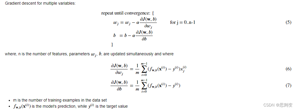
多变量损失函数：

多变量梯度下降实现：

多变量梯度实现：

多变量梯度下降实现：

之前部分实现的梯度下降线性预测模型中的training example只有一个特征属性：房屋面积，这显然是不符合实际情况的，这里增加特征属性的数量再实现一次梯度下降线性预测模型。

这里回顾一下梯度下降线性模型的实现方法：

实现线性模型：f = w*x + b，模型参数w,b待定
寻找最优的w,b组合：

（1）引入衡量模型优劣的cost function：J(w,b) ——损失函数或者代价函数

（2）损失函数值最小的时候，模型最接近实际情况：通过梯度下降法来寻找最优w,b组合

模型初始化信息：

新的房子的特征有：房子面积、卧室数、楼层数、房龄共4个特征属性。

Size (sqft)	Number of Bedrooms	Number of floors	Age of Home	Price (1000s dollars)
2104	5	1	45	460
1416	3	2	40	232
852	2	1	35	17

上面表中的训练样本有3个，输入特征矩阵模型为：

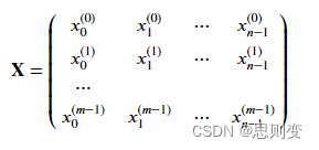
具体代码实现为，X_train是输入矩阵，y_train是输出矩阵

X_train = np.array([[2104, 5, 1, 45], 
                    [1416, 3, 2, 40],
                    [852, 2, 1, 35]])
y_train = np.array([460, 232, 178])

模型参数w,b矩阵：

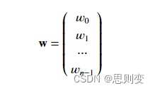
代码实现：w中的每一个元素对应房屋的一个特征属性

b_init = 785.1811367994083
w_init = np.array([ 0.39133535, 18.75376741, -53.36032453, -26.42131618])

模型实现：

def predict(x, w, b): 
    """
    single predict using linear regression
    Args:
      x (ndarray): Shape (n,) example with multiple features
      w (ndarray): Shape (n,) model parameters   
      b (scalar):             model parameter 
      
    Returns:
      p (scalar):  prediction
    """
    p = np.dot(x, w) + b     
    return p

多变量损失函数：

J(w,b)为：

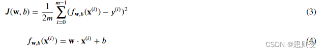
代码实现为:

def compute_cost(X, y, w, b): 
    """
    compute cost
    Args:
      X (ndarray (m,n)): Data, m examples with n features
      y (ndarray (m,)) : target values
      w (ndarray (n,)) : model parameters  
      b (scalar)       : model parameter
      
    Returns:
      cost (scalar): cost
    """
    m = X.shape[0]
    cost = 0.0
    for i in range(m):                                
        f_wb_i = np.dot(X[i], w) + b           #(n,)(n,) = scalar (see np.dot)
        cost = cost + (f_wb_i - y[i])**2       #scalar
    cost = cost / (2 * m)                      #scalar    
    return cost

多变量梯度下降实现：

多变量梯度实现：

def compute_gradient(X, y, w, b): 
    """
    Computes the gradient for linear regression 
    Args:
      X (ndarray (m,n)): Data, m examples with n features
      y (ndarray (m,)) : target values
      w (ndarray (n,)) : model parameters  
      b (scalar)       : model parameter
      
    Returns:
      dj_dw (ndarray (n,)): The gradient of the cost w.r.t. the parameters w. 
      dj_db (scalar):       The gradient of the cost w.r.t. the parameter b. 
    """
    m,n = X.shape           #(number of examples, number of features)
    dj_dw = np.zeros((n,))
    dj_db = 0.

    for i in range(m):                             
        err = (np.dot(X[i], w) + b) - y[i]   
        for j in range(n):                         
            dj_dw[j] = dj_dw[j] + err * X[i, j]    
        dj_db = dj_db + err                        
    dj_dw = dj_dw / m                                
    dj_db = dj_db / m                                
        
    return dj_db, dj_dw

多变量梯度下降实现：

def gradient_descent(X, y, w_in, b_in, cost_function, gradient_function, alpha, num_iters): 
    """
    Performs batch gradient descent to learn theta. Updates theta by taking 
    num_iters gradient steps with learning rate alpha
    
    Args:
      X (ndarray (m,n))   : Data, m examples with n features
      y (ndarray (m,))    : target values
      w_in (ndarray (n,)) : initial model parameters  
      b_in (scalar)       : initial model parameter
      cost_function       : function to compute cost
      gradient_function   : function to compute the gradient
      alpha (float)       : Learning rate
      num_iters (int)     : number of iterations to run gradient descent
      
    Returns:
      w (ndarray (n,)) : Updated values of parameters 
      b (scalar)       : Updated value of parameter 
      """
    
    # An array to store cost J and w's at each iteration primarily for graphing later
    J_history = []
    w = copy.deepcopy(w_in)  #avoid modifying global w within function
    b = b_in
    
    for i in range(num_iters):

        # Calculate the gradient and update the parameters
        dj_db,dj_dw = gradient_function(X, y, w, b)   ##None

        # Update Parameters using w, b, alpha and gradient
        w = w - alpha * dj_dw               ##None
        b = b - alpha * dj_db               ##None
      
        # Save cost J at each iteration
        if i<100000:      # prevent resource exhaustion 
            J_history.append( cost_function(X, y, w, b))

        # Print cost every at intervals 10 times or as many iterations if < 10
        if i% math.ceil(num_iters / 10) == 0:
            print(f"Iteration {i:4d}: Cost {J_history[-1]:8.2f}   ")
        
    return w, b, J_history #return final w,b and J history for graphing

梯度下降算法测试：

# initialize parameters
initial_w = np.zeros_like(w_init)
initial_b = 0.
# some gradient descent settings
iterations = 1000
alpha = 5.0e-7
# run gradient descent 
w_final, b_final, J_hist = gradient_descent(X_train, y_train, initial_w, initial_b,
                                                    compute_cost, compute_gradient, 
                                                    alpha, iterations)
print(f"b,w found by gradient descent: {b_final:0.2f},{w_final} ")
m,_ = X_train.shape
for i in range(m):
    print(f"prediction: {np.dot(X_train[i], w_final) + b_final:0.2f}, target value: {y_train[i]}")


# plot cost versus iteration  
fig, (ax1, ax2) = plt.subplots(1, 2, constrained_layout=True, figsize=(12, 4))
ax1.plot(J_hist)
ax2.plot(100 + np.arange(len(J_hist[100:])), J_hist[100:])
ax1.set_title("Cost vs. iteration");  ax2.set_title("Cost vs. iteration (tail)")
ax1.set_ylabel('Cost')             ;  ax2.set_ylabel('Cost') 
ax1.set_xlabel('iteration step')   ;  ax2.set_xlabel('iteration step') 
plt.show()

结果为：

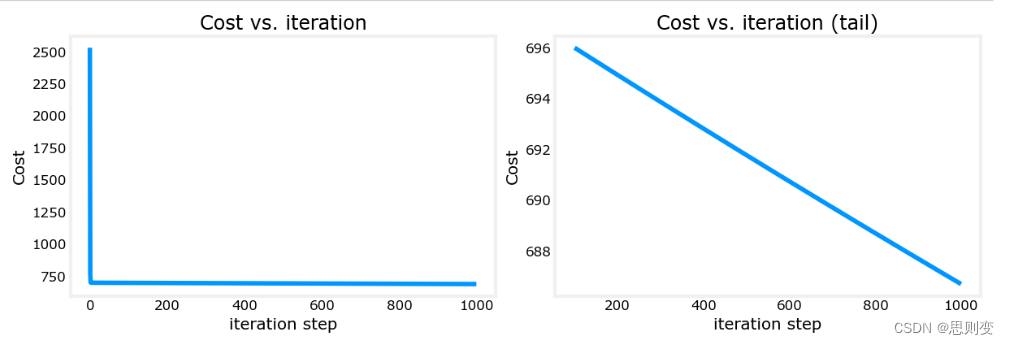
可以看到，右图中损失函数在traning次数结束之后还一直在下降，没有找到最佳的w,b组合。具体解决方法，后面会有更新。

完整的代码为：

import copy, math
import numpy as np
import matplotlib.pyplot as plt

np.set_printoptions(precision=2)  # reduced display precision on numpy arrays

X_train = np.array([[2104, 5, 1, 45], [1416, 3, 2, 40], [852, 2, 1, 35]])
y_train = np.array([460, 232, 178])

b_init = 785.1811367994083
w_init = np.array([ 0.39133535, 18.75376741, -53.36032453, -26.42131618])


def predict(x, w, b):
    """
    single predict using linear regression
    Args:
      x (ndarray): Shape (n,) example with multiple features
      w (ndarray): Shape (n,) model parameters
      b (scalar):             model parameter

    Returns:
      p (scalar):  prediction
    """
    p = np.dot(x, w) + b
    return p


def compute_cost(X, y, w, b):
    """
    compute cost
    Args:
      X (ndarray (m,n)): Data, m examples with n features
      y (ndarray (m,)) : target values
      w (ndarray (n,)) : model parameters
      b (scalar)       : model parameter

    Returns:
      cost (scalar): cost
    """
    m = X.shape[0]
    cost = 0.0
    for i in range(m):
        f_wb_i = np.dot(X[i], w) + b  # (n,)(n,) = scalar (see np.dot)
        cost = cost + (f_wb_i - y[i]) ** 2  # scalar
    cost = cost / (2 * m)  # scalar
    return cost


def compute_gradient(X, y, w, b):
    """
    Computes the gradient for linear regression
    Args:
      X (ndarray (m,n)): Data, m examples with n features
      y (ndarray (m,)) : target values
      w (ndarray (n,)) : model parameters
      b (scalar)       : model parameter

    Returns:
      dj_dw (ndarray (n,)): The gradient of the cost w.r.t. the parameters w.
      dj_db (scalar):       The gradient of the cost w.r.t. the parameter b.
    """
    m, n = X.shape  # (number of examples, number of features)
    dj_dw = np.zeros((n,))
    dj_db = 0.

    for i in range(m):
        err = (np.dot(X[i], w) + b) - y[i]
        for j in range(n):
            dj_dw[j] = dj_dw[j] + err * X[i, j]
        dj_db = dj_db + err
    dj_dw = dj_dw / m
    dj_db = dj_db / m

    return dj_db, dj_dw


def gradient_descent(X, y, w_in, b_in, cost_function, gradient_function, alpha, num_iters):
    """
    Performs batch gradient descent to learn theta. Updates theta by taking
    num_iters gradient steps with learning rate alpha

    Args:
      X (ndarray (m,n))   : Data, m examples with n features
      y (ndarray (m,))    : target values
      w_in (ndarray (n,)) : initial model parameters
      b_in (scalar)       : initial model parameter
      cost_function       : function to compute cost
      gradient_function   : function to compute the gradient
      alpha (float)       : Learning rate
      num_iters (int)     : number of iterations to run gradient descent

    Returns:
      w (ndarray (n,)) : Updated values of parameters
      b (scalar)       : Updated value of parameter
      """

    # An array to store cost J and w's at each iteration primarily for graphing later
    J_history = []
    w = copy.deepcopy(w_in)  # avoid modifying global w within function
    b = b_in

    for i in range(num_iters):

        # Calculate the gradient and update the parameters
        dj_db, dj_dw = gradient_function(X, y, w, b)  ##None

        # Update Parameters using w, b, alpha and gradient
        w = w - alpha * dj_dw  ##None
        b = b - alpha * dj_db  ##None

        # Save cost J at each iteration
        if i < 100000:  # prevent resource exhaustion
            J_history.append(cost_function(X, y, w, b))

        # Print cost every at intervals 10 times or as many iterations if < 10
        if i % math.ceil(num_iters / 10) == 0:
            print(f"Iteration {i:4d}: Cost {J_history[-1]:8.2f}   ")

    return w, b, J_history  # return final w,b and J history for graphing

# initialize parameters
initial_w = np.zeros_like(w_init)
initial_b = 0.
# some gradient descent settings
iterations = 1000
alpha = 5.0e-7
# run gradient descent
w_final, b_final, J_hist = gradient_descent(X_train, y_train, initial_w, initial_b,
                                                    compute_cost, compute_gradient,
                                                    alpha, iterations)
print(f"b,w found by gradient descent: {b_final:0.2f},{w_final} ")
m,_ = X_train.shape
for i in range(m):
    print(f"prediction: {np.dot(X_train[i], w_final) + b_final:0.2f}, target value: {y_train[i]}")

# plot cost versus iteration
fig, (ax1, ax2) = plt.subplots(1, 2, constrained_layout=True, figsize=(12, 4))
ax1.plot(J_hist)
ax2.plot(100 + np.arange(len(J_hist[100:])), J_hist[100:])
ax1.set_title("Cost vs. iteration");  ax2.set_title("Cost vs. iteration (tail)")
ax1.set_ylabel('Cost')             ;  ax2.set_ylabel('Cost')
ax1.set_xlabel('iteration step')   ;  ax2.set_xlabel('iteration step')
plt.show()