Overfitting and Regularization
- 1. 过拟合
- 添加正则化
- 2. 具有正则化的损失函数
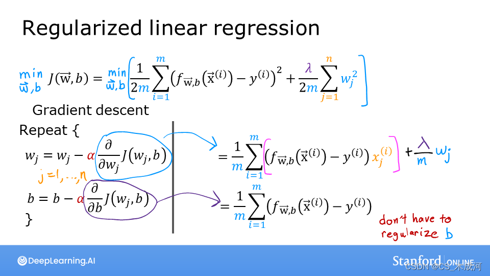
- 2.1 正则化线性回归的损失函数
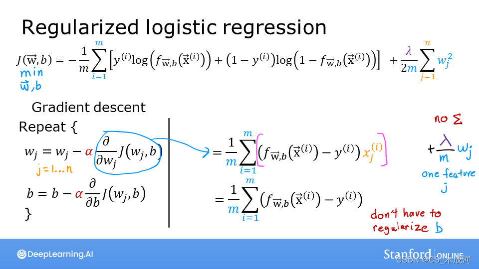
- 2.2 正则化逻辑回归的损失函数
- 3. 具有正则化的梯度下降
- 3.1 使用正则化计算梯度(线性回归 / 逻辑回归)
- 3.2 正则化线性回归的梯度函数
- 3.3 正则化逻辑回归的梯度函数
- 4. 重新运行过拟合示例
- 附录
导入所需的库
import numpy as np
%matplotlib inline
import matplotlib.pyplot as plt
from ipywidgets import Output
from plt_overfit import overfit_example, output
from lab_utils_common import sigmoid
plt.style.use('./deeplearning.mplstyle')
np.set_printoptions(precision=8)
1. 过拟合
plt.close("all")
display(output)
ofit = overfit_example(False)
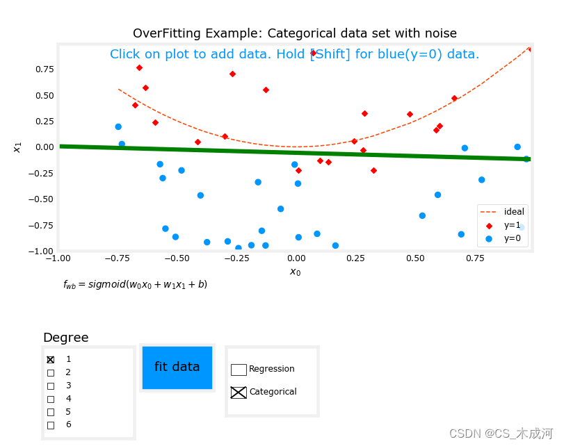
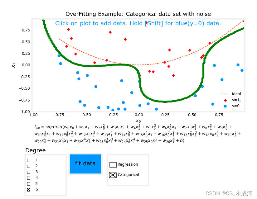
从图中可以看出,拟合度= 1的数据;为“欠拟合”。拟合度= 6的数据;为“过拟合”
添加正则化
线性回归和逻辑回归之间的损失函数存在差异,但在方程中添加正则化是相同的。
线性回归和逻辑回归的梯度函数非常相似。它们的区别仅在于
f
w
b
f_{wb}
fwb 的实现。
2. 具有正则化的损失函数
2.1 正则化线性回归的损失函数
正则化线性回归的损失函数等式表示为:
J
(
w
,
b
)
=
1
2
m
∑
i
=
0
m
−
1
(
f
w
,
b
(
x
(
i
)
)
−
y
(
i
)
)
2
+
λ
2
m
∑
j
=
0
n
−
1
w
j
2
(1)
J(\mathbf{w},b) = \frac{1}{2m} \sum\limits_{i = 0}^{m-1} (f_{\mathbf{w},b}(\mathbf{x}^{(i)}) - y^{(i)})^2 + \frac{\lambda}{2m} \sum_{j=0}^{n-1} w_j^2 \tag{1}
J(w,b)=2m1i=0∑m−1(fw,b(x(i))−y(i))2+2mλj=0∑n−1wj2(1)
其中,
f
w
,
b
(
x
(
i
)
)
=
w
⋅
x
(
i
)
+
b
(2)
f_{\mathbf{w},b}(\mathbf{x}^{(i)}) = \mathbf{w} \cdot \mathbf{x}^{(i)} + b \tag{2}
fw,b(x(i))=w⋅x(i)+b(2)
与没有正则化的线性回归相比,区别在于正则化项,即: λ 2 m ∑ j = 0 n − 1 w j 2 \frac{\lambda}{2m} \sum_{j=0}^{n-1} w_j^2 2mλ∑j=0n−1wj2
带有正则化可以激励梯度下降最小化参数的大小。需要注意的是,在这个例子中,参数 b b b没有被正则化,这是标准做法。
等式(1)和(2)的实现如下:
def compute_cost_linear_reg(X, y, w, b, lambda_ = 1):
    """
    Computes the cost over all examples
    Args:
      X (ndarray (m,n): Data, m examples with n features
      y (ndarray (m,)): target values
      w (ndarray (n,)): model parameters
      b (scalar)      : model parameter
      lambda_ (scalar): Controls amount of regularization
    Returns:
      total_cost (scalar):  cost
    """

    m  = X.shape[0]
    n  = len(w)
    cost = 0.
    for i in range(m):
        f_wb_i = np.dot(X[i], w) + b                                   #(n,)(n,)=scalar, see np.dot
        cost = cost + (f_wb_i - y[i])**2                               #scalar
    cost = cost / (2 * m)                                              #scalar

    reg_cost = 0
    for j in range(n):
        reg_cost += (w[j]**2)                                          #scalar
    reg_cost = (lambda_/(2*m)) * reg_cost                              #scalar

    total_cost = cost + reg_cost                                       #scalar
    return total_cost                                                  #scalar
np.random.seed(1)
X_tmp = np.random.rand(5,6)
y_tmp = np.array([0,1,0,1,0])
w_tmp = np.random.rand(X_tmp.shape[1]).reshape(-1,)-0.5
b_tmp = 0.5
lambda_tmp = 0.7
cost_tmp = compute_cost_linear_reg(X_tmp, y_tmp, w_tmp, b_tmp, lambda_tmp)

print("Regularized cost:", cost_tmp)

2.2 正则化逻辑回归的损失函数
对于正则化的逻辑回归,损失函数表示为:
J
(
w
,
b
)
=
1
m
∑
i
=
0
m
−
1
[
−
y
(
i
)
log
(
f
w
,
b
(
x
(
i
)
)
)
−
(
1
−
y
(
i
)
)
log
(
1
−
f
w
,
b
(
x
(
i
)
)
)
]
+
λ
2
m
∑
j
=
0
n
−
1
w
j
2
(3)
J(\mathbf{w},b) = \frac{1}{m} \sum_{i=0}^{m-1} \left[ -y^{(i)} \log\left(f_{\mathbf{w},b}\left( \mathbf{x}^{(i)} \right) \right) - \left( 1 - y^{(i)}\right) \log \left( 1 - f_{\mathbf{w},b}\left( \mathbf{x}^{(i)} \right) \right) \right] + \frac{\lambda}{2m} \sum_{j=0}^{n-1} w_j^2 \tag{3}
J(w,b)=m1i=0∑m−1[−y(i)log(fw,b(x(i)))−(1−y(i))log(1−fw,b(x(i)))]+2mλj=0∑n−1wj2(3)
其中,
f
w
,
b
(
x
(
i
)
)
=
s
i
g
m
o
i
d
(
w
⋅
x
(
i
)
+
b
)
(4)
f_{\mathbf{w},b}(\mathbf{x}^{(i)}) = sigmoid(\mathbf{w} \cdot \mathbf{x}^{(i)} + b) \tag{4}
fw,b(x(i))=sigmoid(w⋅x(i)+b)(4)
同样,与没有正则化的逻辑回归相比,区别在于正则化项,即: λ 2 m ∑ j = 0 n − 1 w j 2 \frac{\lambda}{2m} \sum_{j=0}^{n-1} w_j^2 2mλ∑j=0n−1wj2
代码实现为:
def compute_cost_logistic_reg(X, y, w, b, lambda_ = 1):
    """
    Computes the cost over all examples
    Args:
    Args:
      X (ndarray (m,n): Data, m examples with n features
      y (ndarray (m,)): target values
      w (ndarray (n,)): model parameters
      b (scalar)      : model parameter
      lambda_ (scalar): Controls amount of regularization
    Returns:
      total_cost (scalar):  cost
    """

    m,n  = X.shape
    cost = 0.
    for i in range(m):
        z_i = np.dot(X[i], w) + b                                      #(n,)(n,)=scalar, see np.dot
        f_wb_i = sigmoid(z_i)                                          #scalar
        cost +=  -y[i]*np.log(f_wb_i) - (1-y[i])*np.log(1-f_wb_i)      #scalar

    cost = cost/m                                                      #scalar

    reg_cost = 0
    for j in range(n):
        reg_cost += (w[j]**2)                                          #scalar
    reg_cost = (lambda_/(2*m)) * reg_cost                              #scalar

    total_cost = cost + reg_cost                                       #scalar
    return total_cost                                                  #scalar
np.random.seed(1)
X_tmp = np.random.rand(5,6)
y_tmp = np.array([0,1,0,1,0])
w_tmp = np.random.rand(X_tmp.shape[1]).reshape(-1,)-0.5
b_tmp = 0.5
lambda_tmp = 0.7
cost_tmp = compute_cost_logistic_reg(X_tmp, y_tmp, w_tmp, b_tmp, lambda_tmp)

print("Regularized cost:", cost_tmp)

3. 具有正则化的梯度下降
运行梯度下降的基本算法不会随着正则化发生改变,正则化改变的是计算梯度。
3.1 使用正则化计算梯度(线性回归 / 逻辑回归)
线性回归和逻辑回归的梯度计算几乎相同,只是在
f
w
b
f_{\mathbf{w}b}
fwb的计算上有所不同。
∂
J
(
w
,
b
)
∂
w
j
=
1
m
∑
i
=
0
m
−
1
(
f
w
,
b
(
x
(
i
)
)
−
y
(
i
)
)
x
j
(
i
)
+
λ
m
w
j
∂
J
(
w
,
b
)
∂
b
=
1
m
∑
i
=
0
m
−
1
(
f
w
,
b
(
x
(
i
)
)
−
y
(
i
)
)
\begin{align*} \frac{\partial J(\mathbf{w},b)}{\partial w_j} &= \frac{1}{m} \sum\limits_{i = 0}^{m-1} (f_{\mathbf{w},b}(\mathbf{x}^{(i)}) - y^{(i)})x_{j}^{(i)} + \frac{\lambda}{m} w_j \tag{2} \\ \frac{\partial J(\mathbf{w},b)}{\partial b} &= \frac{1}{m} \sum\limits_{i = 0}^{m-1} (f_{\mathbf{w},b}(\mathbf{x}^{(i)}) - y^{(i)}) \tag{3} \end{align*}
∂wj∂J(w,b)∂b∂J(w,b)=m1i=0∑m−1(fw,b(x(i))−y(i))xj(i)+mλwj=m1i=0∑m−1(fw,b(x(i))−y(i))(2)(3)
- 对于线性回归模型,
f w , b ( x ) = w ⋅ x + b f_{\mathbf{w},b}(x) = \mathbf{w} \cdot \mathbf{x} + b fw,b(x)=w⋅x+b - 对于逻辑回归模型,
z = w ⋅ x + b z = \mathbf{w} \cdot \mathbf{x} + b z=w⋅x+b
f w , b ( x ) = g ( z ) f_{\mathbf{w},b}(x) = g(z) fw,b(x)=g(z)
其中, g ( z ) g(z) g(z) 是sigmoid 函数:
g ( z ) = 1 1 + e − z g(z) = \frac{1}{1+e^{-z}} g(z)=1+e−z1
添加正则化的项是 λ m w j \frac{\lambda}{m} w_j mλwj
3.2 正则化线性回归的梯度函数
def compute_gradient_linear_reg(X, y, w, b, lambda_):
    """
    Computes the gradient for linear regression
    Args:
      X (ndarray (m,n): Data, m examples with n features
      y (ndarray (m,)): target values
      w (ndarray (n,)): model parameters
      b (scalar)      : model parameter
      lambda_ (scalar): Controls amount of regularization

    Returns:
      dj_dw (ndarray (n,)): The gradient of the cost w.r.t. the parameters w.
      dj_db (scalar):       The gradient of the cost w.r.t. the parameter b.
    """
    m,n = X.shape           #(number of examples, number of features)
    dj_dw = np.zeros((n,))
    dj_db = 0.

    for i in range(m):
        err = (np.dot(X[i], w) + b) - y[i]
        for j in range(n):
            dj_dw[j] = dj_dw[j] + err * X[i, j]
        dj_db = dj_db + err
    dj_dw = dj_dw / m
    dj_db = dj_db / m

    for j in range(n):
        dj_dw[j] = dj_dw[j] + (lambda_/m) * w[j]

    return dj_db, dj_dw
np.random.seed(1)
X_tmp = np.random.rand(5,3)
y_tmp = np.array([0,1,0,1,0])
w_tmp = np.random.rand(X_tmp.shape[1])
b_tmp = 0.5
lambda_tmp = 0.7
dj_db_tmp, dj_dw_tmp = compute_gradient_linear_reg(X_tmp, y_tmp, w_tmp, b_tmp, lambda_tmp)
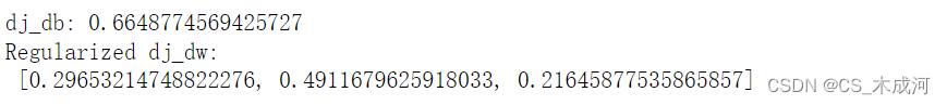
print(f"dj_db: {dj_db_tmp}", )
print(f"Regularized dj_dw:\n {dj_dw_tmp.tolist()}", )
3.3 正则化逻辑回归的梯度函数
def compute_gradient_logistic_reg(X, y, w, b, lambda_):
    """
    Computes the gradient for linear regression

    Args:
      X (ndarray (m,n): Data, m examples with n features
      y (ndarray (m,)): target values
      w (ndarray (n,)): model parameters
      b (scalar)      : model parameter
      lambda_ (scalar): Controls amount of regularization
    Returns
      dj_dw (ndarray Shape (n,)): The gradient of the cost w.r.t. the parameters w.
      dj_db (scalar)            : The gradient of the cost w.r.t. the parameter b.
    """
    m,n = X.shape
    dj_dw = np.zeros((n,))                            #(n,)
    dj_db = 0.0                                       #scalar

    for i in range(m):
        f_wb_i = sigmoid(np.dot(X[i],w) + b)          #(n,)(n,)=scalar
        err_i  = f_wb_i  - y[i]                       #scalar
        for j in range(n):
            dj_dw[j] = dj_dw[j] + err_i * X[i,j]      #scalar
        dj_db = dj_db + err_i
    dj_dw = dj_dw/m                                   #(n,)
    dj_db = dj_db/m                                   #scalar

    for j in range(n):
        dj_dw[j] = dj_dw[j] + (lambda_/m) * w[j]

    return dj_db, dj_dw
np.random.seed(1)
X_tmp = np.random.rand(5,3)
y_tmp = np.array([0,1,0,1,0])
w_tmp = np.random.rand(X_tmp.shape[1])
b_tmp = 0.5
lambda_tmp = 0.7
dj_db_tmp, dj_dw_tmp =  compute_gradient_logistic_reg(X_tmp, y_tmp, w_tmp, b_tmp, lambda_tmp)

print(f"dj_db: {dj_db_tmp}", )
print(f"Regularized dj_dw:\n {dj_dw_tmp.tolist()}", )

4. 重新运行过拟合示例
plt.close("all")
display(output)
ofit = overfit_example(True)
以分类任务(逻辑回归)为例,将拟合度设置为6,
λ
\lambda
λ为0(没有正则化),开始拟合数据,出现了过拟合现象。
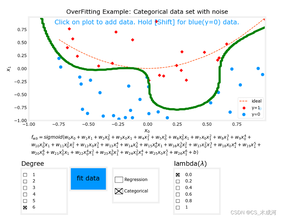
现在,将
λ
\lambda
λ为1(增加正则化),开始拟合数据。
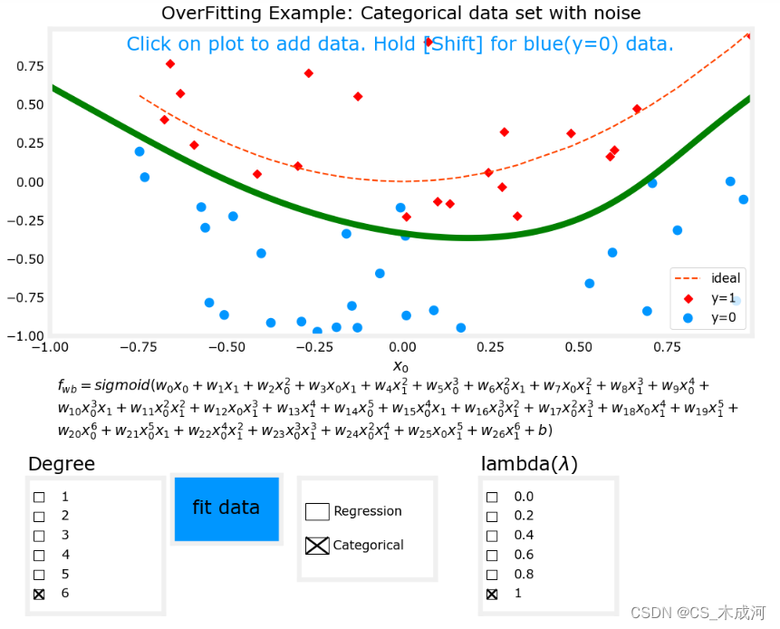
很明显,增加正则化能够减小过拟合。
附录
plot_overfit.py 源码:
"""
plot_overfit
    class and assocaited routines that plot an interactive example of overfitting and its solutions
"""
import math
from ipywidgets import Output
from matplotlib.gridspec import GridSpec
from matplotlib.widgets import Button, CheckButtons
from sklearn.linear_model import LogisticRegression, Ridge
from lab_utils_common import np, plt, dlc, predict_logistic, plot_data, zscore_normalize_features

def map_one_feature(X1, degree):
    """
    Feature mapping function to polynomial features
    """
    X1 = np.atleast_1d(X1)
    out = []
    string = ""
    k = 0
    for i in range(1, degree+1):
        out.append((X1**i))
        string = string + f"w_{{{k}}}{munge('x_0',i)} + "
        k += 1
    string = string + ' b' #add b to text equation, not to data
    return np.stack(out, axis=1), string


def map_feature(X1, X2, degree):
    """
    Feature mapping function to polynomial features
    """
    X1 = np.atleast_1d(X1)
    X2 = np.atleast_1d(X2)

    out = []
    string = ""
    k = 0
    for i in range(1, degree+1):
        for j in range(i + 1):
            out.append((X1**(i-j) * (X2**j)))
            string = string + f"w_{{{k}}}{munge('x_0',i-j)}{munge('x_1',j)} + "
            k += 1
    #print(string + 'b')
    return np.stack(out, axis=1), string + ' b'

def munge(base, exp):
    if exp == 0:
        return ''
    if exp == 1:
        return base
    return base + f'^{{{exp}}}'

def plot_decision_boundary(ax, x0r,x1r, predict,  w, b, scaler = False, mu=None, sigma=None, degree=None):
    """
    Plots a decision boundary
     Args:
      x0r : (array_like Shape (1,1)) range (min, max) of x0
      x1r : (array_like Shape (1,1)) range (min, max) of x1
      predict : function to predict z values
      scalar : (boolean) scale data or not
    """

    h = .01  # step size in the mesh
    # create a mesh to plot in
    xx, yy = np.meshgrid(np.arange(x0r[0], x0r[1], h),
                         np.arange(x1r[0], x1r[1], h))

    # Plot the decision boundary. For that, we will assign a color to each
    # point in the mesh [x_min, m_max]x[y_min, y_max].
    points = np.c_[xx.ravel(), yy.ravel()]
    Xm,_ = map_feature(points[:, 0], points[:, 1],degree)
    if scaler:
        Xm = (Xm - mu)/sigma
    Z = predict(Xm, w, b)

    # Put the result into a color plot
    Z = Z.reshape(xx.shape)
    contour = ax.contour(xx, yy, Z, levels = [0.5], colors='g')
    return contour

# use this to test the above routine
def plot_decision_boundary_sklearn(x0r, x1r, predict, degree,  scaler = False):
    """
    Plots a decision boundary
     Args:
      x0r : (array_like Shape (1,1)) range (min, max) of x0
      x1r : (array_like Shape (1,1)) range (min, max) of x1
      degree: (int)                  degree of polynomial
      predict : function to predict z values
      scaler  : not sure
    """

    h = .01  # step size in the mesh
    # create a mesh to plot in
    xx, yy = np.meshgrid(np.arange(x0r[0], x0r[1], h),
                         np.arange(x1r[0], x1r[1], h))

    # Plot the decision boundary. For that, we will assign a color to each
    # point in the mesh [x_min, m_max]x[y_min, y_max].
    points = np.c_[xx.ravel(), yy.ravel()]
    Xm = map_feature(points[:, 0], points[:, 1],degree)
    if scaler:
        Xm = scaler.transform(Xm)
    Z = predict(Xm)

    # Put the result into a color plot
    Z = Z.reshape(xx.shape)
    plt.contour(xx, yy, Z, colors='g')
    #plot_data(X_train,y_train)

#for debug, uncomment the #@output statments below for routines you want to get error output from
# In the notebook that will call these routines, import  `output`
# from plt_overfit import overfit_example, output
# then, in a cell where the error messages will be the output of..
#display(output)

output = Output() # sends hidden error messages to display when using widgets

class button_manager:
    ''' Handles some missing features of matplotlib check buttons
    on init:
        creates button, links to button_click routine,
        calls call_on_click with active index and firsttime=True
    on click:
        maintains single button on state, calls call_on_click
    '''

    @output.capture()  # debug
    def __init__(self,fig, dim, labels, init, call_on_click):
        '''
        dim: (list)     [leftbottom_x,bottom_y,width,height]
        labels: (list)  for example ['1','2','3','4','5','6']
        init: (list)    for example [True, False, False, False, False, False]
        '''
        self.fig = fig
        self.ax = plt.axes(dim)  #lx,by,w,h
        self.init_state = init
        self.call_on_click = call_on_click
        self.button  = CheckButtons(self.ax,labels,init)
        self.button.on_clicked(self.button_click)
        self.status = self.button.get_status()
        self.call_on_click(self.status.index(True),firsttime=True)

    @output.capture()  # debug
    def reinit(self):
        self.status = self.init_state
        self.button.set_active(self.status.index(True))      #turn off old, will trigger update and set to status

    @output.capture()  # debug
    def button_click(self, event):
        ''' maintains one-on state. If on-button is clicked, will process correctly '''
        #new_status = self.button.get_status()
        #new = [self.status[i] ^ new_status[i] for i in range(len(self.status))]
        #newidx = new.index(True)
        self.button.eventson = False
        self.button.set_active(self.status.index(True))  #turn off old or reenable if same
        self.button.eventson = True
        self.status = self.button.get_status()
        self.call_on_click(self.status.index(True))

class overfit_example():
    """ plot overfit example """
    # pylint: disable=too-many-instance-attributes
    # pylint: disable=too-many-locals
    # pylint: disable=missing-function-docstring
    # pylint: disable=attribute-defined-outside-init
    def __init__(self, regularize=False):
        self.regularize=regularize
        self.lambda_=0
        fig = plt.figure( figsize=(8,6))
        fig.canvas.toolbar_visible = False
        fig.canvas.header_visible = False
        fig.canvas.footer_visible = False
        fig.set_facecolor('#ffffff') #white
        gs  = GridSpec(5, 3, figure=fig)
        ax0 = fig.add_subplot(gs[0:3, :])
        ax1 = fig.add_subplot(gs[-2, :])
        ax2 = fig.add_subplot(gs[-1, :])
        ax1.set_axis_off()
        ax2.set_axis_off()
        self.ax = [ax0,ax1,ax2]
        self.fig = fig

        self.axfitdata = plt.axes([0.26,0.124,0.12,0.1 ])  #lx,by,w,h
        self.bfitdata  = Button(self.axfitdata , 'fit data', color=dlc['dlblue'])
        self.bfitdata.label.set_fontsize(12)
        self.bfitdata.on_clicked(self.fitdata_clicked)

        #clear data is a future enhancement
        #self.axclrdata = plt.axes([0.26,0.06,0.12,0.05 ])  #lx,by,w,h
        #self.bclrdata  = Button(self.axclrdata , 'clear data', color='white')
        #self.bclrdata.label.set_fontsize(12)
        #self.bclrdata.on_clicked(self.clrdata_clicked)

        self.cid = fig.canvas.mpl_connect('button_press_event', self.add_data)

        self.typebut = button_manager(fig, [0.4, 0.07,0.15,0.15], ["Regression", "Categorical"],
                                       [False,True], self.toggle_type)

        self.fig.text(0.1, 0.02+0.21, "Degree", fontsize=12)
        self.degrbut = button_manager(fig,[0.1,0.02,0.15,0.2 ], ['1','2','3','4','5','6'],
                                        [True, False, False, False, False, False], self.update_equation)
        if self.regularize:
            self.fig.text(0.6, 0.02+0.21, r"lambda($\lambda$)", fontsize=12)
            self.lambut = button_manager(fig,[0.6,0.02,0.15,0.2 ], ['0.0','0.2','0.4','0.6','0.8','1'],
                                        [True, False, False, False, False, False], self.updt_lambda)

        #self.regbut =  button_manager(fig, [0.8, 0.08,0.24,0.15], ["Regularize"],
        #                               [False], self.toggle_reg)
        #self.logistic_data()

    def updt_lambda(self, idx, firsttime=False):
      # pylint: disable=unused-argument
        self.lambda_ = idx * 0.2

    def toggle_type(self, idx, firsttime=False):
        self.logistic = idx==1
        self.ax[0].clear()
        if self.logistic:
            self.logistic_data()
        else:
            self.linear_data()
        if not firsttime:
            self.degrbut.reinit()

    @output.capture()  # debug
    def logistic_data(self,redraw=False):
        if not redraw:
            m = 50
            n = 2
            np.random.seed(2)
            X_train = 2*(np.random.rand(m,n)-[0.5,0.5])
            y_train = X_train[:,1]+0.5  > X_train[:,0]**2 + 0.5*np.random.rand(m) #quadratic + random
            y_train = y_train + 0  #convert from boolean to integer
            self.X = X_train
            self.y = y_train
            self.x_ideal = np.sort(X_train[:,0])
            self.y_ideal =  self.x_ideal**2


        self.ax[0].plot(self.x_ideal, self.y_ideal, "--", color = "orangered", label="ideal", lw=1)
        plot_data(self.X, self.y, self.ax[0], s=10, loc='lower right')
        self.ax[0].set_title("OverFitting Example: Categorical data set with noise")
        self.ax[0].text(0.5,0.93, "Click on plot to add data. Hold [Shift] for blue(y=0) data.",
                        fontsize=12, ha='center',transform=self.ax[0].transAxes, color=dlc["dlblue"])
        self.ax[0].set_xlabel(r"$x_0$")
        self.ax[0].set_ylabel(r"$x_1$")

    def linear_data(self,redraw=False):
        if not redraw:
            m = 30
            c = 0
            x_train = np.arange(0,m,1)
            np.random.seed(1)
            y_ideal = x_train**2 + c
            y_train = y_ideal + 0.7 * y_ideal*(np.random.sample((m,))-0.5)
            self.x_ideal = x_train #for redraw when new data included in X
            self.X = x_train
            self.y = y_train
            self.y_ideal = y_ideal
        else:
            self.ax[0].set_xlim(self.xlim)
            self.ax[0].set_ylim(self.ylim)

        self.ax[0].scatter(self.X,self.y, label="y")
        self.ax[0].plot(self.x_ideal, self.y_ideal, "--", color = "orangered", label="y_ideal", lw=1)
        self.ax[0].set_title("OverFitting Example: Regression Data Set (quadratic with noise)",fontsize = 14)
        self.ax[0].set_xlabel("x")
        self.ax[0].set_ylabel("y")
        self.ax0ledgend = self.ax[0].legend(loc='lower right')
        self.ax[0].text(0.5,0.93, "Click on plot to add data",
                        fontsize=12, ha='center',transform=self.ax[0].transAxes, color=dlc["dlblue"])
        if not redraw:
            self.xlim = self.ax[0].get_xlim()
            self.ylim = self.ax[0].get_ylim()


    @output.capture()  # debug
    def add_data(self, event):
        if self.logistic:
            self.add_data_logistic(event)
        else:
            self.add_data_linear(event)

    @output.capture()  # debug
    def add_data_logistic(self, event):
        if event.inaxes == self.ax[0]:
            x0_coord = event.xdata
            x1_coord = event.ydata

            if event.key is None:  #shift not pressed
                self.ax[0].scatter(x0_coord, x1_coord, marker='x', s=10, c = 'red', label="y=1")
                self.y = np.append(self.y,1)
            else:
                self.ax[0].scatter(x0_coord, x1_coord, marker='o', s=10, label="y=0", facecolors='none',
                                   edgecolors=dlc['dlblue'],lw=3)
                self.y = np.append(self.y,0)
            self.X = np.append(self.X,np.array([[x0_coord, x1_coord]]),axis=0)
        self.fig.canvas.draw()

    def add_data_linear(self, event):
        if event.inaxes == self.ax[0]:
            x_coord = event.xdata
            y_coord = event.ydata

            self.ax[0].scatter(x_coord, y_coord, marker='o', s=10, facecolors='none',
                                   edgecolors=dlc['dlblue'],lw=3)
            self.y = np.append(self.y,y_coord)
            self.X = np.append(self.X,x_coord)
            self.fig.canvas.draw()

    #@output.capture()  # debug
    #def clrdata_clicked(self,event):
    #    if self.logistic == True:
    #        self.X = np.
    #    else:
    #        self.linear_regression()


    @output.capture()  # debug
    def fitdata_clicked(self,event):
        if self.logistic:
            self.logistic_regression()
        else:
            self.linear_regression()

    def linear_regression(self):
        self.ax[0].clear()
        self.fig.canvas.draw()

        # create and fit the model using our mapped_X feature set.
        self.X_mapped, _ =  map_one_feature(self.X, self.degree)
        self.X_mapped_scaled, self.X_mu, self.X_sigma  = zscore_normalize_features(self.X_mapped)

        #linear_model = LinearRegression()
        linear_model = Ridge(alpha=self.lambda_, normalize=True, max_iter=10000)
        linear_model.fit(self.X_mapped_scaled, self.y )
        self.w = linear_model.coef_.reshape(-1,)
        self.b = linear_model.intercept_
        x = np.linspace(*self.xlim,30)  #plot line idependent of data which gets disordered
        xm, _ =  map_one_feature(x, self.degree)
        xms = (xm - self.X_mu)/ self.X_sigma
        y_pred = linear_model.predict(xms)

        #self.fig.canvas.draw()
        self.linear_data(redraw=True)
        self.ax0yfit = self.ax[0].plot(x, y_pred, color = "blue", label="y_fit")
        self.ax0ledgend = self.ax[0].legend(loc='lower right')
        self.fig.canvas.draw()

    def logistic_regression(self):
        self.ax[0].clear()
        self.fig.canvas.draw()

        # create and fit the model using our mapped_X feature set.
        self.X_mapped, _ =  map_feature(self.X[:, 0], self.X[:, 1], self.degree)
        self.X_mapped_scaled, self.X_mu, self.X_sigma  = zscore_normalize_features(self.X_mapped)
        if not self.regularize or self.lambda_ == 0:
            lr = LogisticRegression(penalty='none', max_iter=10000)
        else:
            C = 1/self.lambda_
            lr = LogisticRegression(C=C, max_iter=10000)

        lr.fit(self.X_mapped_scaled,self.y)
        #print(lr.score(self.X_mapped_scaled, self.y))
        self.w = lr.coef_.reshape(-1,)
        self.b = lr.intercept_
        #print(self.w, self.b)
        self.logistic_data(redraw=True)
        self.contour = plot_decision_boundary(self.ax[0],[-1,1],[-1,1], predict_logistic, self.w, self.b,
                       scaler=True, mu=self.X_mu, sigma=self.X_sigma, degree=self.degree )
        self.fig.canvas.draw()

    @output.capture()  # debug
    def update_equation(self, idx, firsttime=False):
        #print(f"Update equation, index = {idx}, firsttime={firsttime}")
        self.degree = idx+1
        if firsttime:
            self.eqtext = []
        else:
            for artist in self.eqtext:
                #print(artist)
                artist.remove()
            self.eqtext = []
        if self.logistic:
            _, equation =  map_feature(self.X[:, 0], self.X[:, 1], self.degree)
            string = 'f_{wb} = sigmoid('
        else:
            _, equation =  map_one_feature(self.X, self.degree)
            string = 'f_{wb} = ('
        bz = 10
        seq = equation.split('+')
        blks = math.ceil(len(seq)/bz)
        for i in range(blks):
            if i == 0:
                string = string +  '+'.join(seq[bz*i:bz*i+bz])
            else:
                string = '+'.join(seq[bz*i:bz*i+bz])
            string = string + ')' if i == blks-1 else string + '+'
            ei = self.ax[1].text(0.01,(0.75-i*0.25), f"${string}$",fontsize=9,
                                 transform = self.ax[1].transAxes, ma='left', va='top' )
            self.eqtext.append(ei)
        self.fig.canvas.draw()