导入所需的库

import copy, math
import numpy as np
%matplotlib widget
import matplotlib.pyplot as plt
from lab_utils_common import  dlc, plot_data, plt_tumor_data, sigmoid, compute_cost_logistic
from plt_quad_logistic import plt_quad_logistic, plt_prob
plt.style.use('./deeplearning.mplstyle')

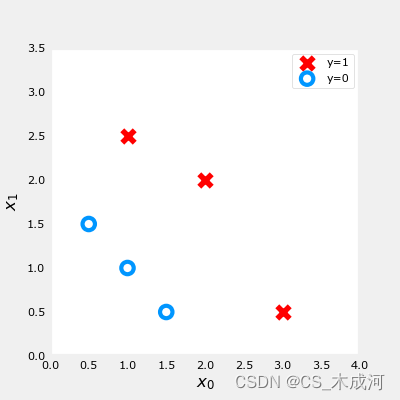
1. 数据集（多变量）

X_train = np.array([[0.5, 1.5], [1,1], [1.5, 0.5], [3, 0.5], [2, 2], [1, 2.5]])
y_train = np.array([0, 0, 0, 1, 1, 1])

fig,ax = plt.subplots(1,1,figsize=(4,4))
plot_data(X_train, y_train, ax)

ax.axis([0, 4, 0, 3.5])
ax.set_ylabel('$x_1$', fontsize=12)
ax.set_xlabel('$x_0$', fontsize=12)
plt.show()

2. 逻辑梯度下降

梯度下降计算公式:
repeat until convergence:    {        w j = w j − α ∂ J ( w , b ) ∂ w j    for j := 0..n-1            b = b − α ∂ J ( w , b ) ∂ b } \begin{align*} &\text{repeat until convergence:} \; \lbrace \\ & \; \; \;w_j = w_j - \alpha \frac{\partial J(\mathbf{w},b)}{\partial w_j} \tag{1} \; & \text{for j := 0..n-1} \\ & \; \; \; \; \;b = b - \alpha \frac{\partial J(\mathbf{w},b)}{\partial b} \\ &\rbrace \end{align*} ​repeat until convergence:{wj​=wj​−α∂wj​∂J(w,b)​b=b−α∂b∂J(w,b)​}​for j := 0..n-1(1)​

其中，对于所有的 $j$ 每次迭代同时更新 $w_j$ ,
$$\begin{array}{rl}\frac{\partial J(\mathbf{w},b)}{\partial w_j}& =\frac{1}{m}\sum _{i=0}^{m-1}(f_{\mathbf{w},b}({\mathbf{x}}^{(i)})-y^{(i)})x_j^{(i)}\\ \frac{\partial J(\mathbf{w},b)}{\partial b}& =\frac{1}{m}\sum _{i=0}^{m-1}(f_{\mathbf{w},b}({\mathbf{x}}^{(i)})-y^{(i)})\end{array}\text{\hspace{1em}(2)(3)}$$

• m 是训练集样例的数量
• $f_{\mathbf{w},b}(x^{(i)})$ 是模型预测值, $y^{(i)}$ 是目标值
• 对于逻辑回归模型
  $z=\mathbf{w}\cdot \mathbf{x}+b$
  $f_{\mathbf{w},b}(x)=g(z)$
  其中 $g(z)$ 是 sigmoid 函数： $g(z)=\frac{1}{1+e^{-z}}$

3. 梯度下降的实现及代码描述

实现梯度下降算法需要两步：

• 循环实现上面等式(1). 即下面的 gradient_descent
• 当前梯度的计算等式(2, 3). 即下面的 compute_gradient_logistic

3.1 计算梯度

对于所有的$w_j$ 和 $b$，实现等式 (2),(3)

• 初始化变量计算 dj_dw 和 dj_db

• 对每个样例：

  • 计算误差 $g(\mathbf{w}\cdot {\mathbf{x}}^{(i)}+b)-{\mathbf{y}}^{(i)}$
  • 对于这个样例中的每个输入值 $x_j^{(i)}$ ,
    • 误差乘以输入值 $x_j^{(i)}$, 然后加到对应的 dj_dw 中. (上述等式2)
  • 累加误差到 dj_db (上述等式3)

• dj_db 和 dj_dw都除以样例总数$m$

• 在Numpy中${\mathbf{x}}^{(i)}$ 是 X[i,:] 或者X[i] ， $x_j^{(i)}$ 是 X[i,j]

代码描述：

def compute_gradient_logistic(X, y, w, b): 
    """
    Computes the gradient for linear regression 
 
    Args:
      X (ndarray (m,n): Data, m examples with n features
      y (ndarray (m,)): target values
      w (ndarray (n,)): model parameters  
      b (scalar)      : model parameter
    Returns
      dj_dw (ndarray (n,)): The gradient of the cost w.r.t. the parameters w. 
      dj_db (scalar)      : The gradient of the cost w.r.t. the parameter b. 
    """
    m,n = X.shape
    dj_dw = np.zeros((n,))                           #(n,)
    dj_db = 0.

    for i in range(m):
        f_wb_i = sigmoid(np.dot(X[i],w) + b)          #(n,)(n,)=scalar
        err_i  = f_wb_i  - y[i]                       #scalar
        for j in range(n):
            dj_dw[j] = dj_dw[j] + err_i * X[i,j]      #scalar
        dj_db = dj_db + err_i
    dj_dw = dj_dw/m                                   #(n,)
    dj_db = dj_db/m                                   #scalar
        
    return dj_db, dj_dw  

测试一下

X_tmp = np.array([[0.5, 1.5], [1,1], [1.5, 0.5], [3, 0.5], [2, 2], [1, 2.5]])
y_tmp = np.array([0, 0, 0, 1, 1, 1])
w_tmp = np.array([2.,3.])
b_tmp = 1.
dj_db_tmp, dj_dw_tmp = compute_gradient_logistic(X_tmp, y_tmp, w_tmp, b_tmp)
print(f"dj_db: {dj_db_tmp}" )
print(f"dj_dw: {dj_dw_tmp.tolist()}" )

3.2 梯度下降

实现上述公式(1)，代码为：

def gradient_descent(X, y, w_in, b_in, alpha, num_iters): 
    """
    Performs batch gradient descent
    
    Args:
      X (ndarray (m,n)   : Data, m examples with n features
      y (ndarray (m,))   : target values
      w_in (ndarray (n,)): Initial values of model parameters  
      b_in (scalar)      : Initial values of model parameter
      alpha (float)      : Learning rate
      num_iters (scalar) : number of iterations to run gradient descent
      
    Returns:
      w (ndarray (n,))   : Updated values of parameters
      b (scalar)         : Updated value of parameter 
    """
    # An array to store cost J and w's at each iteration primarily for graphing later
    J_history = []
    w = copy.deepcopy(w_in)  #avoid modifying global w within function
    b = b_in
    
    for i in range(num_iters):
        # Calculate the gradient and update the parameters
        dj_db, dj_dw = compute_gradient_logistic(X, y, w, b)   

        # Update Parameters using w, b, alpha and gradient
        w = w - alpha * dj_dw               
        b = b - alpha * dj_db               
      
        # Save cost J at each iteration
        if i<100000:      # prevent resource exhaustion 
            J_history.append( compute_cost_logistic(X, y, w, b) )

        # Print cost every at intervals 10 times or as many iterations if < 10
        if i% math.ceil(num_iters / 10) == 0:
            print(f"Iteration {i:4d}: Cost {J_history[-1]}   ")
        
    return w, b, J_history         #return final w,b and J history for graphing

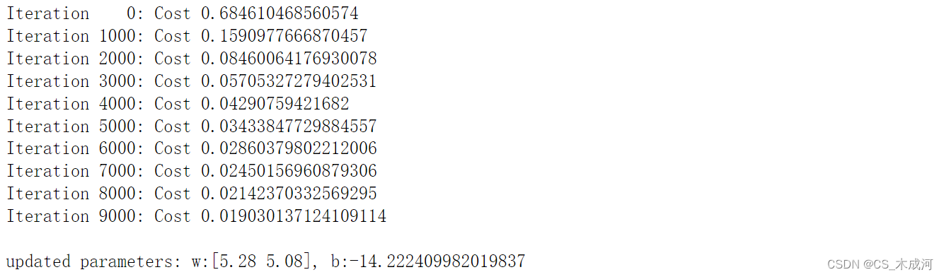
运行一下：

w_tmp  = np.zeros_like(X_train[0])
b_tmp  = 0.
alph = 0.1
iters = 10000

w_out, b_out, _ = gradient_descent(X_train, y_train, w_tmp, b_tmp, alph, iters) 
print(f"\nupdated parameters: w:{w_out}, b:{b_out}")

梯度下降的结果可视化：

fig,ax = plt.subplots(1,1,figsize=(5,4))
# plot the probability 
plt_prob(ax, w_out, b_out)

# Plot the original data
ax.set_ylabel(r'$x_1$')
ax.set_xlabel(r'$x_0$')   
ax.axis([0, 4, 0, 3.5])
plot_data(X_train,y_train,ax)

# Plot the decision boundary
x0 = -b_out/w_out[1]
x1 = -b_out/w_out[0]
ax.plot([0,x0],[x1,0], c=dlc["dlblue"], lw=1)
plt.show()

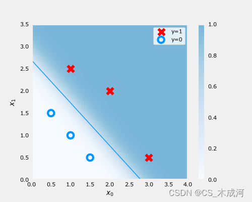
在上图中，阴影部分表示概率 y=1，决策边界是概率为0.5的直线。

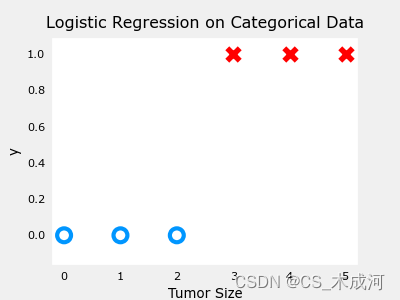
4. 数据集（单变量）

导入数据绘图可视化，此时参数为$w$, $b$：

x_train = np.array([0., 1, 2, 3, 4, 5])
y_train = np.array([0,  0, 0, 1, 1, 1])

fig,ax = plt.subplots(1,1,figsize=(4,3))
plt_tumor_data(x_train, y_train, ax)
plt.show()

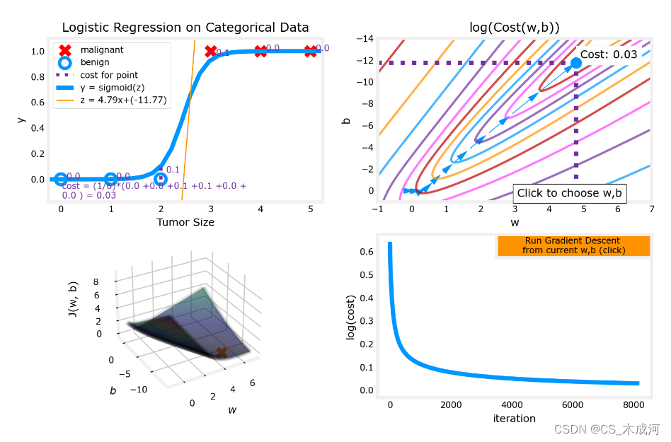
w_range = np.array([-1, 7])
b_range = np.array([1, -14])
quad = plt_quad_logistic( x_train, y_train, w_range, b_range )

附录

lab_utils_common.py 源码：

"""
lab_utils_common
   contains common routines and variable definitions
   used by all the labs in this week.
   by contrast, specific, large plotting routines will be in separate files
   and are generally imported into the week where they are used.
   those files will import this file
"""
import copy
import math
import numpy as np
import matplotlib.pyplot as plt
from matplotlib.patches import FancyArrowPatch
from ipywidgets import Output

np.set_printoptions(precision=2)

dlc = dict(dlblue = '#0096ff', dlorange = '#FF9300', dldarkred='#C00000', dlmagenta='#FF40FF', dlpurple='#7030A0')
dlblue = '#0096ff'; dlorange = '#FF9300'; dldarkred='#C00000'; dlmagenta='#FF40FF'; dlpurple='#7030A0'
dlcolors = [dlblue, dlorange, dldarkred, dlmagenta, dlpurple]
plt.style.use('./deeplearning.mplstyle')

def sigmoid(z):
    """
    Compute the sigmoid of z

    Parameters
    ----------
    z : array_like
        A scalar or numpy array of any size.

    Returns
    -------
     g : array_like
         sigmoid(z)
    """
    z = np.clip( z, -500, 500 )           # protect against overflow
    g = 1.0/(1.0+np.exp(-z))

    return g

##########################################################
# Regression Routines
##########################################################

def predict_logistic(X, w, b):
    """ performs prediction """
    return sigmoid(X @ w + b)

def predict_linear(X, w, b):
    """ performs prediction """
    return X @ w + b

def compute_cost_logistic(X, y, w, b, lambda_=0, safe=False):
    """
    Computes cost using logistic loss, non-matrix version

    Args:
      X (ndarray): Shape (m,n)  matrix of examples with n features
      y (ndarray): Shape (m,)   target values
      w (ndarray): Shape (n,)   parameters for prediction
      b (scalar):               parameter  for prediction
      lambda_ : (scalar, float) Controls amount of regularization, 0 = no regularization
      safe : (boolean)          True-selects under/overflow safe algorithm
    Returns:
      cost (scalar): cost
    """

    m,n = X.shape
    cost = 0.0
    for i in range(m):
        z_i    = np.dot(X[i],w) + b                                             #(n,)(n,) or (n,) ()
        if safe:  #avoids overflows
            cost += -(y[i] * z_i ) + log_1pexp(z_i)
        else:
            f_wb_i = sigmoid(z_i)                                                   #(n,)
            cost  += -y[i] * np.log(f_wb_i) - (1 - y[i]) * np.log(1 - f_wb_i)       # scalar
    cost = cost/m

    reg_cost = 0
    if lambda_ != 0:
        for j in range(n):
            reg_cost += (w[j]**2)                                               # scalar
        reg_cost = (lambda_/(2*m))*reg_cost

    return cost + reg_cost


def log_1pexp(x, maximum=20):
    ''' approximate log(1+exp^x)
        https://stats.stackexchange.com/questions/475589/numerical-computation-of-cross-entropy-in-practice
    Args:
    x   : (ndarray Shape (n,1) or (n,)  input
    out : (ndarray Shape matches x      output ~= np.log(1+exp(x))
    '''

    out  = np.zeros_like(x,dtype=float)
    i    = x <= maximum
    ni   = np.logical_not(i)

    out[i]  = np.log(1 + np.exp(x[i]))
    out[ni] = x[ni]
    return out


def compute_cost_matrix(X, y, w, b, logistic=False, lambda_=0, safe=True):
    """
    Computes the cost using  using matrices
    Args:
      X : (ndarray, Shape (m,n))          matrix of examples
      y : (ndarray  Shape (m,) or (m,1))  target value of each example
      w : (ndarray  Shape (n,) or (n,1))  Values of parameter(s) of the model
      b : (scalar )                       Values of parameter of the model
      verbose : (Boolean) If true, print out intermediate value f_wb
    Returns:
      total_cost: (scalar)                cost
    """
    m = X.shape[0]
    y = y.reshape(-1,1)             # ensure 2D
    w = w.reshape(-1,1)             # ensure 2D
    if logistic:
        if safe:  #safe from overflow
            z = X @ w + b                                                           #(m,n)(n,1)=(m,1)
            cost = -(y * z) + log_1pexp(z)
            cost = np.sum(cost)/m                                                   # (scalar)
        else:
            f    = sigmoid(X @ w + b)                                               # (m,n)(n,1) = (m,1)
            cost = (1/m)*(np.dot(-y.T, np.log(f)) - np.dot((1-y).T, np.log(1-f)))   # (1,m)(m,1) = (1,1)
            cost = cost[0,0]                                                        # scalar
    else:
        f    = X @ w + b                                                        # (m,n)(n,1) = (m,1)
        cost = (1/(2*m)) * np.sum((f - y)**2)                                   # scalar

    reg_cost = (lambda_/(2*m)) * np.sum(w**2)                                   # scalar

    total_cost = cost + reg_cost                                                # scalar

    return total_cost                                                           # scalar

def compute_gradient_matrix(X, y, w, b, logistic=False, lambda_=0):
    """
    Computes the gradient using matrices

    Args:
      X : (ndarray, Shape (m,n))          matrix of examples
      y : (ndarray  Shape (m,) or (m,1))  target value of each example
      w : (ndarray  Shape (n,) or (n,1))  Values of parameters of the model
      b : (scalar )                       Values of parameter of the model
      logistic: (boolean)                 linear if false, logistic if true
      lambda_:  (float)                   applies regularization if non-zero
    Returns
      dj_dw: (array_like Shape (n,1))     The gradient of the cost w.r.t. the parameters w
      dj_db: (scalar)                     The gradient of the cost w.r.t. the parameter b
    """
    m = X.shape[0]
    y = y.reshape(-1,1)             # ensure 2D
    w = w.reshape(-1,1)             # ensure 2D

    f_wb  = sigmoid( X @ w + b ) if logistic else  X @ w + b      # (m,n)(n,1) = (m,1)
    err   = f_wb - y                                              # (m,1)
    dj_dw = (1/m) * (X.T @ err)                                   # (n,m)(m,1) = (n,1)
    dj_db = (1/m) * np.sum(err)                                   # scalar

    dj_dw += (lambda_/m) * w        # regularize                  # (n,1)

    return dj_db, dj_dw                                           # scalar, (n,1)

def gradient_descent(X, y, w_in, b_in, alpha, num_iters, logistic=False, lambda_=0, verbose=True):
    """
    Performs batch gradient descent to learn theta. Updates theta by taking
    num_iters gradient steps with learning rate alpha

    Args:
      X (ndarray):    Shape (m,n)         matrix of examples
      y (ndarray):    Shape (m,) or (m,1) target value of each example
      w_in (ndarray): Shape (n,) or (n,1) Initial values of parameters of the model
      b_in (scalar):                      Initial value of parameter of the model
      logistic: (boolean)                 linear if false, logistic if true
      lambda_:  (float)                   applies regularization if non-zero
      alpha (float):                      Learning rate
      num_iters (int):                    number of iterations to run gradient descent

    Returns:
      w (ndarray): Shape (n,) or (n,1)    Updated values of parameters; matches incoming shape
      b (scalar):                         Updated value of parameter
    """
    # An array to store cost J and w's at each iteration primarily for graphing later
    J_history = []
    w = copy.deepcopy(w_in)  #avoid modifying global w within function
    b = b_in
    w = w.reshape(-1,1)      #prep for matrix operations
    y = y.reshape(-1,1)

    for i in range(num_iters):

        # Calculate the gradient and update the parameters
        dj_db,dj_dw = compute_gradient_matrix(X, y, w, b, logistic, lambda_)

        # Update Parameters using w, b, alpha and gradient
        w = w - alpha * dj_dw
        b = b - alpha * dj_db

        # Save cost J at each iteration
        if i<100000:      # prevent resource exhaustion
            J_history.append( compute_cost_matrix(X, y, w, b, logistic, lambda_) )

        # Print cost every at intervals 10 times or as many iterations if < 10
        if i% math.ceil(num_iters / 10) == 0:
            if verbose: print(f"Iteration {i:4d}: Cost {J_history[-1]}   ")

    return w.reshape(w_in.shape), b, J_history  #return final w,b and J history for graphing

def zscore_normalize_features(X):
    """
    computes  X, zcore normalized by column

    Args:
      X (ndarray): Shape (m,n) input data, m examples, n features

    Returns:
      X_norm (ndarray): Shape (m,n)  input normalized by column
      mu (ndarray):     Shape (n,)   mean of each feature
      sigma (ndarray):  Shape (n,)   standard deviation of each feature
    """
    # find the mean of each column/feature
    mu     = np.mean(X, axis=0)                 # mu will have shape (n,)
    # find the standard deviation of each column/feature
    sigma  = np.std(X, axis=0)                  # sigma will have shape (n,)
    # element-wise, subtract mu for that column from each example, divide by std for that column
    X_norm = (X - mu) / sigma

    return X_norm, mu, sigma

#check our work
#from sklearn.preprocessing import scale
#scale(X_orig, axis=0, with_mean=True, with_std=True, copy=True)

######################################################
# Common Plotting Routines
######################################################


def plot_data(X, y, ax, pos_label="y=1", neg_label="y=0", s=80, loc='best' ):
    """ plots logistic data with two axis """
    # Find Indices of Positive and Negative Examples
    pos = y == 1
    neg = y == 0
    pos = pos.reshape(-1,)  #work with 1D or 1D y vectors
    neg = neg.reshape(-1,)

    # Plot examples
    ax.scatter(X[pos, 0], X[pos, 1], marker='x', s=s, c = 'red', label=pos_label)
    ax.scatter(X[neg, 0], X[neg, 1], marker='o', s=s, label=neg_label, facecolors='none', edgecolors=dlblue, lw=3)
    ax.legend(loc=loc)

    ax.figure.canvas.toolbar_visible = False
    ax.figure.canvas.header_visible = False
    ax.figure.canvas.footer_visible = False

def plt_tumor_data(x, y, ax):
    """ plots tumor data on one axis """
    pos = y == 1
    neg = y == 0

    ax.scatter(x[pos], y[pos], marker='x', s=80, c = 'red', label="malignant")
    ax.scatter(x[neg], y[neg], marker='o', s=100, label="benign", facecolors='none', edgecolors=dlblue,lw=3)
    ax.set_ylim(-0.175,1.1)
    ax.set_ylabel('y')
    ax.set_xlabel('Tumor Size')
    ax.set_title("Logistic Regression on Categorical Data")

    ax.figure.canvas.toolbar_visible = False
    ax.figure.canvas.header_visible = False
    ax.figure.canvas.footer_visible = False

# Draws a threshold at 0.5
def draw_vthresh(ax,x):
    """ draws a threshold """
    ylim = ax.get_ylim()
    xlim = ax.get_xlim()
    ax.fill_between([xlim[0], x], [ylim[1], ylim[1]], alpha=0.2, color=dlblue)
    ax.fill_between([x, xlim[1]], [ylim[1], ylim[1]], alpha=0.2, color=dldarkred)
    ax.annotate("z >= 0", xy= [x,0.5], xycoords='data',
                xytext=[30,5],textcoords='offset points')
    d = FancyArrowPatch(
        posA=(x, 0.5), posB=(x+3, 0.5), color=dldarkred,
        arrowstyle='simple, head_width=5, head_length=10, tail_width=0.0',
    )
    ax.add_artist(d)
    ax.annotate("z < 0", xy= [x,0.5], xycoords='data',
                 xytext=[-50,5],textcoords='offset points', ha='left')
    f = FancyArrowPatch(
        posA=(x, 0.5), posB=(x-3, 0.5), color=dlblue,
        arrowstyle='simple, head_width=5, head_length=10, tail_width=0.0',
    )
    ax.add_artist(f)

plt_quad_logistic.py 源码：

"""
plt_quad_logistic.py
    interactive plot and supporting routines showing logistic regression
"""

import time
from matplotlib import cm
import matplotlib.colors as colors
from matplotlib.gridspec import GridSpec
from matplotlib.widgets import Button
from matplotlib.patches import FancyArrowPatch
from ipywidgets import Output
from lab_utils_common import np, plt, dlc, dlcolors, sigmoid, compute_cost_matrix, gradient_descent

# for debug
#output = Output() # sends hidden error messages to display when using widgets
#display(output)

class plt_quad_logistic:
    ''' plots a quad plot showing logistic regression '''
    # pylint: disable=too-many-instance-attributes
    # pylint: disable=too-many-locals
    # pylint: disable=missing-function-docstring
    # pylint: disable=attribute-defined-outside-init
    def __init__(self, x_train,y_train, w_range, b_range):
        # setup figure
        fig = plt.figure( figsize=(10,6))
        fig.canvas.toolbar_visible = False
        fig.canvas.header_visible = False
        fig.canvas.footer_visible = False
        fig.set_facecolor('#ffffff') #white
        gs  = GridSpec(2, 2, figure=fig)
        ax0 = fig.add_subplot(gs[0, 0])
        ax1 = fig.add_subplot(gs[0, 1])
        ax2 = fig.add_subplot(gs[1, 0],  projection='3d')
        ax3 = fig.add_subplot(gs[1,1])
        pos = ax3.get_position().get_points()  ##[[lb_x,lb_y], [rt_x, rt_y]]
        h = 0.05 
        width = 0.2
        axcalc   = plt.axes([pos[1,0]-width, pos[1,1]-h, width, h])  #lx,by,w,h
        ax = np.array([ax0, ax1, ax2, ax3, axcalc])
        self.fig = fig
        self.ax = ax
        self.x_train = x_train
        self.y_train = y_train

        self.w = 0. #initial point, non-array
        self.b = 0.

        # initialize subplots
        self.dplot = data_plot(ax[0], x_train, y_train, self.w, self.b)
        self.con_plot = contour_and_surface_plot(ax[1], ax[2], x_train, y_train, w_range, b_range, self.w, self.b)
        self.cplot = cost_plot(ax[3])

        # setup events
        self.cid = fig.canvas.mpl_connect('button_press_event', self.click_contour)
        self.bcalc = Button(axcalc, 'Run Gradient Descent \nfrom current w,b (click)', color=dlc["dlorange"])
        self.bcalc.on_clicked(self.calc_logistic)

#    @output.capture()  # debug
    def click_contour(self, event):
        ''' called when click in contour '''
        if event.inaxes == self.ax[1]:   #contour plot
            self.w = event.xdata
            self.b = event.ydata

            self.cplot.re_init()
            self.dplot.update(self.w, self.b)
            self.con_plot.update_contour_wb_lines(self.w, self.b)
            self.con_plot.path.re_init(self.w, self.b)

            self.fig.canvas.draw()

#    @output.capture()  # debug
    def calc_logistic(self, event):
        ''' called on run gradient event '''
        for it in [1, 8,16,32,64,128,256,512,1024,2048,4096]:
            w, self.b, J_hist = gradient_descent(self.x_train.reshape(-1,1), self.y_train.reshape(-1,1),
                                                 np.array(self.w).reshape(-1,1), self.b, 0.1, it,
                                                 logistic=True, lambda_=0, verbose=False)
            self.w = w[0,0]
            self.dplot.update(self.w, self.b)
            self.con_plot.update_contour_wb_lines(self.w, self.b)
            self.con_plot.path.add_path_item(self.w,self.b)
            self.cplot.add_cost(J_hist)

            time.sleep(0.3)
            self.fig.canvas.draw()


class data_plot:
    ''' handles data plot '''
    # pylint: disable=missing-function-docstring
    # pylint: disable=attribute-defined-outside-init
    def __init__(self, ax, x_train, y_train, w, b):
        self.ax = ax
        self.x_train = x_train
        self.y_train = y_train
        self.m = x_train.shape[0]
        self.w = w
        self.b = b

        self.plt_tumor_data()
        self.draw_logistic_lines(firsttime=True)
        self.mk_cost_lines(firsttime=True)

        self.ax.autoscale(enable=False) # leave plot scales the same after initial setup

    def plt_tumor_data(self):
        x = self.x_train
        y = self.y_train
        pos = y == 1
        neg = y == 0
        self.ax.scatter(x[pos], y[pos], marker='x', s=80, c = 'red', label="malignant")
        self.ax.scatter(x[neg], y[neg], marker='o', s=100, label="benign", facecolors='none',
                   edgecolors=dlc["dlblue"],lw=3)
        self.ax.set_ylim(-0.175,1.1)
        self.ax.set_ylabel('y')
        self.ax.set_xlabel('Tumor Size')
        self.ax.set_title("Logistic Regression on Categorical Data")

    def update(self, w, b):
        self.w = w
        self.b = b
        self.draw_logistic_lines()
        self.mk_cost_lines()

    def draw_logistic_lines(self, firsttime=False):
        if not firsttime:
            self.aline[0].remove()
            self.bline[0].remove()
            self.alegend.remove()

        xlim  = self.ax.get_xlim()
        x_hat = np.linspace(*xlim, 30)
        y_hat = sigmoid(np.dot(x_hat.reshape(-1,1), self.w) + self.b)
        self.aline = self.ax.plot(x_hat, y_hat, color=dlc["dlblue"],
                                     label="y = sigmoid(z)")
        f_wb = np.dot(x_hat.reshape(-1,1), self.w) + self.b
        self.bline = self.ax.plot(x_hat, f_wb, color=dlc["dlorange"], lw=1,
                                     label=f"z = {np.squeeze(self.w):0.2f}x+({self.b:0.2f})")
        self.alegend = self.ax.legend(loc='upper left')

    def mk_cost_lines(self, firsttime=False):
        ''' makes vertical cost lines'''
        if not firsttime:
            for artist in self.cost_items:
                artist.remove()
        self.cost_items = []
        cstr = f"cost = (1/{self.m})*("
        ctot = 0
        label = 'cost for point'
        addedbreak = False
        for p in zip(self.x_train,self.y_train):
            f_wb_p = sigmoid(self.w*p[0]+self.b)
            c_p = compute_cost_matrix(p[0].reshape(-1,1), p[1],np.array(self.w), self.b, logistic=True, lambda_=0, safe=True)
            c_p_txt = c_p
            a = self.ax.vlines(p[0], p[1],f_wb_p, lw=3, color=dlc["dlpurple"], ls='dotted', label=label)
            label='' #just one
            cxy = [p[0], p[1] + (f_wb_p-p[1])/2]
            b = self.ax.annotate(f'{c_p_txt:0.1f}', xy=cxy, xycoords='data',color=dlc["dlpurple"],
                        xytext=(5, 0), textcoords='offset points')
            cstr += f"{c_p_txt:0.1f} +"
            if len(cstr) > 38 and addedbreak is False:
                cstr += "\n"
                addedbreak = True
            ctot += c_p
            self.cost_items.extend((a,b))
        ctot = ctot/(len(self.x_train))
        cstr = cstr[:-1] + f") = {ctot:0.2f}"
        ## todo.. figure out how to get this textbox to extend to the width of the subplot
        c = self.ax.text(0.05,0.02,cstr, transform=self.ax.transAxes, color=dlc["dlpurple"])
        self.cost_items.append(c)


class contour_and_surface_plot:
    ''' plots combined in class as they have similar operations '''
    # pylint: disable=missing-function-docstring
    # pylint: disable=attribute-defined-outside-init
    def __init__(self, axc, axs, x_train, y_train, w_range, b_range, w, b):

        self.x_train = x_train
        self.y_train = y_train
        self.axc = axc
        self.axs = axs

        #setup useful ranges and common linspaces
        b_space  = np.linspace(*b_range, 100)
        w_space  = np.linspace(*w_range, 100)

        # get cost for w,b ranges for contour and 3D
        tmp_b,tmp_w = np.meshgrid(b_space,w_space)
        z = np.zeros_like(tmp_b)
        for i in range(tmp_w.shape[0]):
            for j in range(tmp_w.shape[1]):
                z[i,j] = compute_cost_matrix(x_train.reshape(-1,1), y_train, tmp_w[i,j], tmp_b[i,j],
                                             logistic=True, lambda_=0, safe=True)
                if z[i,j] == 0:
                    z[i,j] = 1e-9

        ### plot contour ###
        CS = axc.contour(tmp_w, tmp_b, np.log(z),levels=12, linewidths=2, alpha=0.7,colors=dlcolors)
        axc.set_title('log(Cost(w,b))')
        axc.set_xlabel('w', fontsize=10)
        axc.set_ylabel('b', fontsize=10)
        axc.set_xlim(w_range)
        axc.set_ylim(b_range)
        self.update_contour_wb_lines(w, b, firsttime=True)
        axc.text(0.7,0.05,"Click to choose w,b",  bbox=dict(facecolor='white', ec = 'black'), fontsize = 10,
                transform=axc.transAxes, verticalalignment = 'center', horizontalalignment= 'center')

        #Surface plot of the cost function J(w,b)
        axs.plot_surface(tmp_w, tmp_b, z,  cmap = cm.jet, alpha=0.3, antialiased=True)
        axs.plot_wireframe(tmp_w, tmp_b, z, color='k', alpha=0.1)
        axs.set_xlabel("$w$")
        axs.set_ylabel("$b$")
        axs.zaxis.set_rotate_label(False)
        axs.xaxis.set_pane_color((1.0, 1.0, 1.0, 0.0))
        axs.yaxis.set_pane_color((1.0, 1.0, 1.0, 0.0))
        axs.zaxis.set_pane_color((1.0, 1.0, 1.0, 0.0))
        axs.set_zlabel("J(w, b)", rotation=90)
        axs.view_init(30, -120)

        axs.autoscale(enable=False)
        axc.autoscale(enable=False)

        self.path = path(self.w,self.b, self.axc)  # initialize an empty path, avoids existance check

    def update_contour_wb_lines(self, w, b, firsttime=False):
        self.w = w
        self.b = b
        cst = compute_cost_matrix(self.x_train.reshape(-1,1), self.y_train, np.array(self.w), self.b,
                                  logistic=True, lambda_=0, safe=True)

        # remove lines and re-add on contour plot and 3d plot
        if not firsttime:
            for artist in self.dyn_items:
                artist.remove()
        a = self.axc.scatter(self.w, self.b, s=100, color=dlc["dlblue"], zorder= 10, label="cost with \ncurrent w,b")
        b = self.axc.hlines(self.b, self.axc.get_xlim()[0], self.w, lw=4, color=dlc["dlpurple"], ls='dotted')
        c = self.axc.vlines(self.w, self.axc.get_ylim()[0] ,self.b, lw=4, color=dlc["dlpurple"], ls='dotted')
        d = self.axc.annotate(f"Cost: {cst:0.2f}", xy= (self.w, self.b), xytext = (4,4), textcoords = 'offset points',
                           bbox=dict(facecolor='white'), size = 10)
        #Add point in 3D surface plot
        e = self.axs.scatter3D(self.w, self.b, cst , marker='X', s=100)

        self.dyn_items = [a,b,c,d,e]


class cost_plot:
    """ manages cost plot for plt_quad_logistic """
    # pylint: disable=missing-function-docstring
    # pylint: disable=attribute-defined-outside-init
    def __init__(self,ax):
        self.ax = ax
        self.ax.set_ylabel("log(cost)")
        self.ax.set_xlabel("iteration")
        self.costs = []
        self.cline = self.ax.plot(0,0, color=dlc["dlblue"])

    def re_init(self):
        self.ax.clear()
        self.__init__(self.ax)

    def add_cost(self,J_hist):
        self.costs.extend(J_hist)
        self.cline[0].remove()
        self.cline = self.ax.plot(self.costs)

class path:
    ''' tracks paths during gradient descent on contour plot '''
    # pylint: disable=missing-function-docstring
    # pylint: disable=attribute-defined-outside-init
    def __init__(self, w, b, ax):
        ''' w, b at start of path '''
        self.path_items = []
        self.w = w
        self.b = b
        self.ax = ax

    def re_init(self, w, b):
        for artist in self.path_items:
            artist.remove()
        self.path_items = []
        self.w = w
        self.b = b

    def add_path_item(self, w, b):
        a = FancyArrowPatch(
            posA=(self.w, self.b), posB=(w, b), color=dlc["dlblue"],
            arrowstyle='simple, head_width=5, head_length=10, tail_width=0.0',
        )
        self.ax.add_artist(a)
        self.path_items.append(a)
        self.w = w
        self.b = b

#-----------
# related to the logistic gradient descent lab
#----------

def truncate_colormap(cmap, minval=0.0, maxval=1.0, n=100):
    """ truncates color map """
    new_cmap = colors.LinearSegmentedColormap.from_list(
        'trunc({n},{a:.2f},{b:.2f})'.format(n=cmap.name, a=minval, b=maxval),
        cmap(np.linspace(minval, maxval, n)))
    return new_cmap

def plt_prob(ax, w_out,b_out):
    """ plots a decision boundary but include shading to indicate the probability """
    #setup useful ranges and common linspaces
    x0_space  = np.linspace(0, 4 , 100)
    x1_space  = np.linspace(0, 4 , 100)

    # get probability for x0,x1 ranges
    tmp_x0,tmp_x1 = np.meshgrid(x0_space,x1_space)
    z = np.zeros_like(tmp_x0)
    for i in range(tmp_x0.shape[0]):
        for j in range(tmp_x1.shape[1]):
            z[i,j] = sigmoid(np.dot(w_out, np.array([tmp_x0[i,j],tmp_x1[i,j]])) + b_out)


    cmap = plt.get_cmap('Blues')
    new_cmap = truncate_colormap(cmap, 0.0, 0.5)
    pcm = ax.pcolormesh(tmp_x0, tmp_x1, z,
                   norm=cm.colors.Normalize(vmin=0, vmax=1),
                   cmap=new_cmap, shading='nearest', alpha = 0.9)
    ax.figure.colorbar(pcm, ax=ax)