Cost Function
- 1、计算 cost
- 2、cost 函数的直观理解
- 3、cost 可视化
- 总结
- 附录
首先,导入所需的库:
import numpy as np
%matplotlib widget
import matplotlib.pyplot as plt
from lab_utils_uni import plt_intuition, plt_stationary, plt_update_onclick, soup_bowl
plt.style.use('./deeplearning.mplstyle')
1、计算 cost
在这里,术语 ‘cost’ 是衡量模型预测房屋目标价格的程度的指标。
具有一个变量的 cost 计算公式为
J
(
w
,
b
)
=
1
2
m
∑
i
=
0
m
−
1
(
f
w
,
b
(
x
(
i
)
)
−
y
(
i
)
)
2
(1)
J(w,b) = \frac{1}{2m} \sum\limits_{i = 0}^{m-1} (f_{w,b}(x^{(i)}) - y^{(i)})^2 \tag{1}
J(w,b)=2m1i=0∑m−1(fw,b(x(i))−y(i))2(1)
其中,
f
w
,
b
(
x
(
i
)
)
=
w
x
(
i
)
+
b
(2)
f_{w,b}(x^{(i)}) = wx^{(i)} + b \tag{2}
fw,b(x(i))=wx(i)+b(2)
- f w , b ( x ( i ) ) f_{w,b}(x^{(i)}) fw,b(x(i)) 是使用参数 w , b w,b w,b 对样例 i i i 的预测。
- ( f w , b ( x ( i ) ) − y ( i ) ) 2 (f_{w,b}(x^{(i)}) -y^{(i)})^2 (fw,b(x(i))−y(i))2 是目标值和预测值之间的平方差。
-
m
m
m 个样例的平方差进行相加,并除以
2m得到 cost, 即 J ( w , b ) J(w,b) J(w,b).
下面的代码通过循环每个样例来计算 cost。
def compute_cost(x, y, w, b):
    """
    Computes the cost function for linear regression.

    Args:
      x (ndarray (m,)): Data, m examples
      y (ndarray (m,)): target values
      w,b (scalar)    : model parameters

    Returns
        total_cost (float): The cost of using w,b as the parameters for linear regression
               to fit the data points in x and y
    """
    # number of training examples
    m = x.shape[0]

    cost_sum = 0
    for i in range(m):
        f_wb = w * x[i] + b
        cost = (f_wb - y[i]) ** 2
        cost_sum = cost_sum + cost
    total_cost = (1 / (2 * m)) * cost_sum

    return total_cost
2、cost 函数的直观理解
我们的目标是找到一个模型 f w , b ( x ) = w x + b f_{w,b}(x) = wx + b fw,b(x)=wx+b,其中 w w w 和 b b b 是参数,用于准确预测给定输入 x x x 的房屋价格。
上述 cost 计算公式(1)显示,如果可以选择 w w w 和 b b b,使得预测值 f w , b ( x ) f_{w,b}(x) fw,b(x) 与目标值 y y y 相匹配,那么 ( f w , b ( x ( i ) ) − y ( i ) ) 2 (f_{w,b}(x^{(i)}) - y^{(i)})^2 (fw,b(x(i))−y(i))2 项将为零,cost 将被最小化。
在之前的博客中,我们已经确定 b = 100 b=100 b=100 是一个最优解,所以让我们将 b b b 设为 100,并专注于 w w w。
plt_intuition(x_train,y_train)
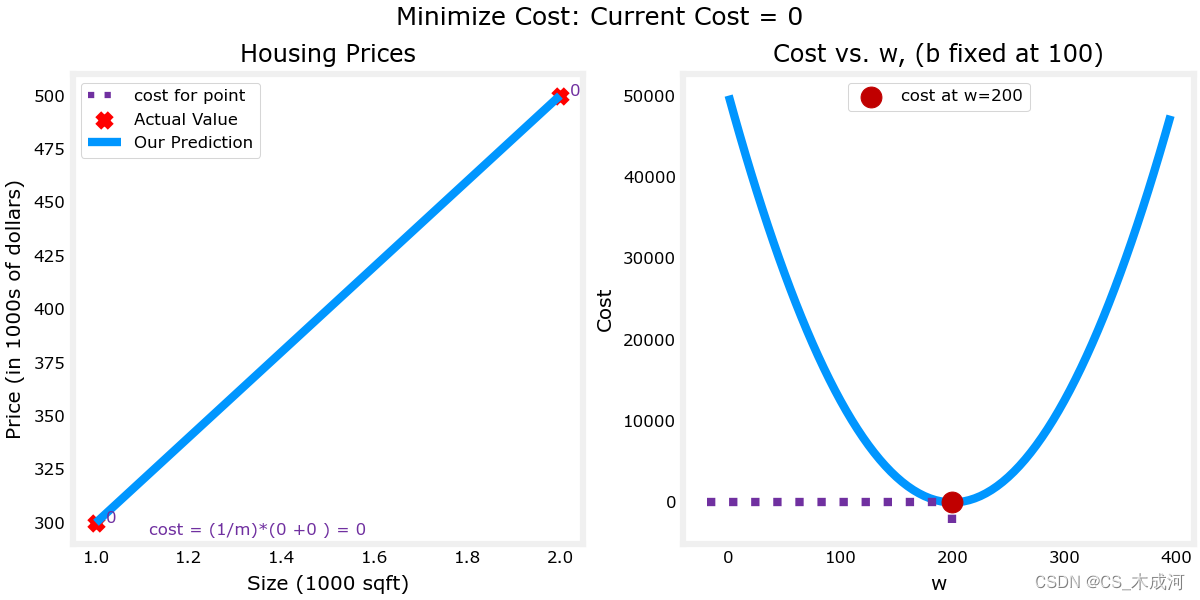
从图中可以就看出:
- 当 𝑤=200 时,cost 被最小化,这与之前博客的结果相匹配。
- 因为在 cost 计算公式中,目标值与预测值之间的差异被平方,所以当 𝑤 太大或太小时,cost 会迅速增加。
- 使用通过最小化 cost 选择的 𝑤 和 𝑏 值得到的直线与数据完美拟合。
3、cost 可视化
我们可以通过绘制3D图或使用等高线图来观察 cost 如何随着同时改变 w 和 b 而变化。
首先,定义更大的数据集
x_train = np.array([1.0, 1.7, 2.0, 2.5, 3.0, 3.2])
y_train = np.array([250, 300, 480,  430,   630, 730,])
plt.close('all')
fig, ax, dyn_items = plt_stationary(x_train, y_train)
updater = plt_update_onclick(fig, ax, x_train, y_train, dyn_items)
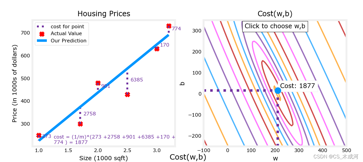
注意,因为我们的训练样例不在一条直线上,所以最小化 cost 不是0。
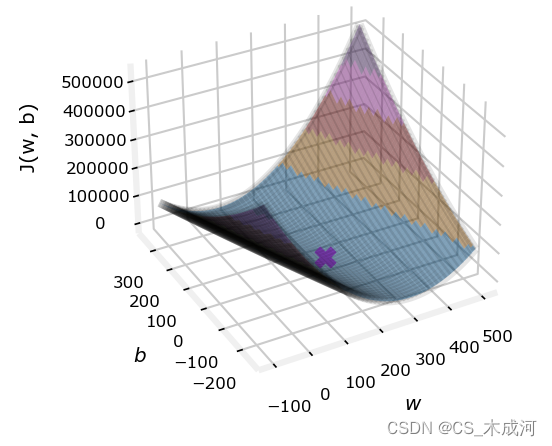
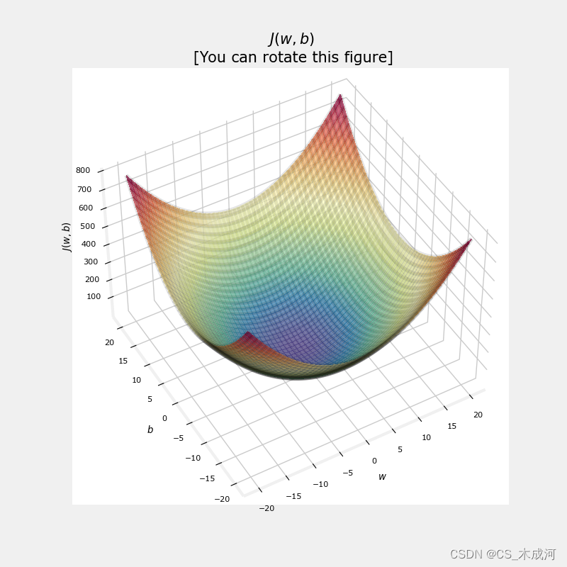
cost 函数对损失进行平方的事实确保了“误差曲面”呈现凸形,就像一个碗一样。它总会有一个通过在所有维度上追随梯度可以到达的最小值点。在之前的图中,由于 w w w 和 b b b 维度的尺度不同,这很难被察觉。下图中的 w w w 和 b b b 是对称的。
soup_bowl()
总结
- cost 计算公式提供了衡量预测与训练数据匹配程度的指标。
- 最小化 cost 可以提供参数 w w w、 b b b 的最优值。
附录
lab_utils_uni.py 源码:
"""
lab_utils_uni.py
    routines used in Course 1, Week2, labs1-3 dealing with single variables (univariate)
"""
import numpy as np
import matplotlib.pyplot as plt
from matplotlib.ticker import MaxNLocator
from matplotlib.gridspec import GridSpec
from matplotlib.colors import LinearSegmentedColormap
from ipywidgets import interact
from lab_utils_common import compute_cost
from lab_utils_common import dlblue, dlorange, dldarkred, dlmagenta, dlpurple, dlcolors

plt.style.use('./deeplearning.mplstyle')
n_bin = 5
dlcm = LinearSegmentedColormap.from_list(
        'dl_map', dlcolors, N=n_bin)

##########################################################
# Plotting Routines
##########################################################

def plt_house_x(X, y,f_wb=None, ax=None):
    ''' plot house with aXis '''
    if not ax:
        fig, ax = plt.subplots(1,1)
    ax.scatter(X, y, marker='x', c='r', label="Actual Value")

    ax.set_title("Housing Prices")
    ax.set_ylabel('Price (in 1000s of dollars)')
    ax.set_xlabel(f'Size (1000 sqft)')
    if f_wb is not None:
        ax.plot(X, f_wb,  c=dlblue, label="Our Prediction")
    ax.legend()


def mk_cost_lines(x,y,w,b, ax):
    ''' makes vertical cost lines'''
    cstr = "cost = (1/m)*("
    ctot = 0
    label = 'cost for point'
    addedbreak = False
    for p in zip(x,y):
        f_wb_p = w*p[0]+b
        c_p = ((f_wb_p - p[1])**2)/2
        c_p_txt = c_p
        ax.vlines(p[0], p[1],f_wb_p, lw=3, color=dlpurple, ls='dotted', label=label)
        label='' #just one
        cxy = [p[0], p[1] + (f_wb_p-p[1])/2]
        ax.annotate(f'{c_p_txt:0.0f}', xy=cxy, xycoords='data',color=dlpurple,
            xytext=(5, 0), textcoords='offset points')
        cstr += f"{c_p_txt:0.0f} +"
        if len(cstr) > 38 and addedbreak is False:
            cstr += "\n"
            addedbreak = True
        ctot += c_p
    ctot = ctot/(len(x))
    cstr = cstr[:-1] + f") = {ctot:0.0f}"
    ax.text(0.15,0.02,cstr, transform=ax.transAxes, color=dlpurple)

##########
# Cost lab
##########


def plt_intuition(x_train, y_train):

    w_range = np.array([200-200,200+200])
    tmp_b = 100

    w_array = np.arange(*w_range, 5)
    cost = np.zeros_like(w_array)
    for i in range(len(w_array)):
        tmp_w = w_array[i]
        cost[i] = compute_cost(x_train, y_train, tmp_w, tmp_b)

    @interact(w=(*w_range,10),continuous_update=False)
    def func( w=150):
        f_wb = np.dot(x_train, w) + tmp_b

        fig, ax = plt.subplots(1, 2, constrained_layout=True, figsize=(8,4))
        fig.canvas.toolbar_position = 'bottom'

        mk_cost_lines(x_train, y_train, w, tmp_b, ax[0])
        plt_house_x(x_train, y_train, f_wb=f_wb, ax=ax[0])

        ax[1].plot(w_array, cost)
        cur_cost = compute_cost(x_train, y_train, w, tmp_b)
        ax[1].scatter(w,cur_cost, s=100, color=dldarkred, zorder= 10, label= f"cost at w={w}")
        ax[1].hlines(cur_cost, ax[1].get_xlim()[0],w, lw=4, color=dlpurple, ls='dotted')
        ax[1].vlines(w, ax[1].get_ylim()[0],cur_cost, lw=4, color=dlpurple, ls='dotted')
        ax[1].set_title("Cost vs. w, (b fixed at 100)")
        ax[1].set_ylabel('Cost')
        ax[1].set_xlabel('w')
        ax[1].legend(loc='upper center')
        fig.suptitle(f"Minimize Cost: Current Cost = {cur_cost:0.0f}", fontsize=12)
        plt.show()

# this is the 2D cost curve with interactive slider
def plt_stationary(x_train, y_train):
    # setup figure
    fig = plt.figure( figsize=(9,8))
    #fig = plt.figure(constrained_layout=True,  figsize=(12,10))
    fig.set_facecolor('#ffffff') #white
    fig.canvas.toolbar_position = 'top'
    #gs = GridSpec(2, 2, figure=fig, wspace = 0.01)
    gs = GridSpec(2, 2, figure=fig)
    ax0 = fig.add_subplot(gs[0, 0])
    ax1 = fig.add_subplot(gs[0, 1])
    ax2 = fig.add_subplot(gs[1, :],  projection='3d')
    ax = np.array([ax0,ax1,ax2])

    #setup useful ranges and common linspaces
    w_range = np.array([200-300.,200+300])
    b_range = np.array([50-300., 50+300])
    b_space  = np.linspace(*b_range, 100)
    w_space  = np.linspace(*w_range, 100)

    # get cost for w,b ranges for contour and 3D
    tmp_b,tmp_w = np.meshgrid(b_space,w_space)
    z=np.zeros_like(tmp_b)
    for i in range(tmp_w.shape[0]):
        for j in range(tmp_w.shape[1]):
            z[i,j] = compute_cost(x_train, y_train, tmp_w[i][j], tmp_b[i][j] )
            if z[i,j] == 0: z[i,j] = 1e-6

    w0=200;b=-100    #initial point
    ### plot model w cost ###
    f_wb = np.dot(x_train,w0) + b
    mk_cost_lines(x_train,y_train,w0,b,ax[0])
    plt_house_x(x_train, y_train, f_wb=f_wb, ax=ax[0])

    ### plot contour ###
    CS = ax[1].contour(tmp_w, tmp_b, np.log(z),levels=12, linewidths=2, alpha=0.7,colors=dlcolors)
    ax[1].set_title('Cost(w,b)')
    ax[1].set_xlabel('w', fontsize=10)
    ax[1].set_ylabel('b', fontsize=10)
    ax[1].set_xlim(w_range) ; ax[1].set_ylim(b_range)
    cscat  = ax[1].scatter(w0,b, s=100, color=dlblue, zorder= 10, label="cost with \ncurrent w,b")
    chline = ax[1].hlines(b, ax[1].get_xlim()[0],w0, lw=4, color=dlpurple, ls='dotted')
    cvline = ax[1].vlines(w0, ax[1].get_ylim()[0],b, lw=4, color=dlpurple, ls='dotted')
    ax[1].text(0.5,0.95,"Click to choose w,b",  bbox=dict(facecolor='white', ec = 'black'), fontsize = 10,
                transform=ax[1].transAxes, verticalalignment = 'center', horizontalalignment= 'center')

    #Surface plot of the cost function J(w,b)
    ax[2].plot_surface(tmp_w, tmp_b, z,  cmap = dlcm, alpha=0.3, antialiased=True)
    ax[2].plot_wireframe(tmp_w, tmp_b, z, color='k', alpha=0.1)
    plt.xlabel("$w$")
    plt.ylabel("$b$")
    ax[2].zaxis.set_rotate_label(False)
    ax[2].xaxis.set_pane_color((1.0, 1.0, 1.0, 0.0))
    ax[2].yaxis.set_pane_color((1.0, 1.0, 1.0, 0.0))
    ax[2].zaxis.set_pane_color((1.0, 1.0, 1.0, 0.0))
    ax[2].set_zlabel("J(w, b)\n\n", rotation=90)
    plt.title("Cost(w,b) \n [You can rotate this figure]", size=12)
    ax[2].view_init(30, -120)

    return fig,ax, [cscat, chline, cvline]


#https://matplotlib.org/stable/users/event_handling.html
class plt_update_onclick:
    def __init__(self, fig, ax, x_train,y_train, dyn_items):
        self.fig = fig
        self.ax = ax
        self.x_train = x_train
        self.y_train = y_train
        self.dyn_items = dyn_items
        self.cid = fig.canvas.mpl_connect('button_press_event', self)

    def __call__(self, event):
        if event.inaxes == self.ax[1]:
            ws = event.xdata
            bs = event.ydata
            cst = compute_cost(self.x_train, self.y_train, ws, bs)

            # clear and redraw line plot
            self.ax[0].clear()
            f_wb = np.dot(self.x_train,ws) + bs
            mk_cost_lines(self.x_train,self.y_train,ws,bs,self.ax[0])
            plt_house_x(self.x_train, self.y_train, f_wb=f_wb, ax=self.ax[0])

            # remove lines and re-add on countour plot and 3d plot
            for artist in self.dyn_items:
                artist.remove()

            a = self.ax[1].scatter(ws,bs, s=100, color=dlblue, zorder= 10, label="cost with \ncurrent w,b")
            b = self.ax[1].hlines(bs, self.ax[1].get_xlim()[0],ws, lw=4, color=dlpurple, ls='dotted')
            c = self.ax[1].vlines(ws, self.ax[1].get_ylim()[0],bs, lw=4, color=dlpurple, ls='dotted')
            d = self.ax[1].annotate(f"Cost: {cst:.0f}", xy= (ws, bs), xytext = (4,4), textcoords = 'offset points',
                               bbox=dict(facecolor='white'), size = 10)

            #Add point in 3D surface plot
            e = self.ax[2].scatter3D(ws, bs,cst , marker='X', s=100)

            self.dyn_items = [a,b,c,d,e]
            self.fig.canvas.draw()


def soup_bowl():
    """ Create figure and plot with a 3D projection"""
    fig = plt.figure(figsize=(8,8))

    #Plot configuration
    ax = fig.add_subplot(111, projection='3d')
    ax.xaxis.set_pane_color((1.0, 1.0, 1.0, 0.0))
    ax.yaxis.set_pane_color((1.0, 1.0, 1.0, 0.0))
    ax.zaxis.set_pane_color((1.0, 1.0, 1.0, 0.0))
    ax.zaxis.set_rotate_label(False)
    ax.view_init(45, -120)

    #Useful linearspaces to give values to the parameters w and b
    w = np.linspace(-20, 20, 100)
    b = np.linspace(-20, 20, 100)

    #Get the z value for a bowl-shaped cost function
    z=np.zeros((len(w), len(b)))
    j=0
    for x in w:
        i=0
        for y in b:
            z[i,j] = x**2 + y**2
            i+=1
        j+=1

    #Meshgrid used for plotting 3D functions
    W, B = np.meshgrid(w, b)

    #Create the 3D surface plot of the bowl-shaped cost function
    ax.plot_surface(W, B, z, cmap = "Spectral_r", alpha=0.7, antialiased=False)
    ax.plot_wireframe(W, B, z, color='k', alpha=0.1)
    ax.set_xlabel("$w$")
    ax.set_ylabel("$b$")
    ax.set_zlabel("$J(w,b)$", rotation=90)
    ax.set_title("$J(w,b)$\n [You can rotate this figure]", size=15)

    plt.show()

def inbounds(a,b,xlim,ylim):
    xlow,xhigh = xlim
    ylow,yhigh = ylim
    ax, ay = a
    bx, by = b
    if (ax > xlow and ax < xhigh) and (bx > xlow and bx < xhigh) \
        and (ay > ylow and ay < yhigh) and (by > ylow and by < yhigh):
        return True
    return False

def plt_contour_wgrad(x, y, hist, ax, w_range=[-100, 500, 5], b_range=[-500, 500, 5],
                contours = [0.1,50,1000,5000,10000,25000,50000],
                      resolution=5, w_final=200, b_final=100,step=10 ):
    b0,w0 = np.meshgrid(np.arange(*b_range),np.arange(*w_range))
    z=np.zeros_like(b0)
    for i in range(w0.shape[0]):
        for j in range(w0.shape[1]):
            z[i][j] = compute_cost(x, y, w0[i][j], b0[i][j] )

    CS = ax.contour(w0, b0, z, contours, linewidths=2,
                   colors=[dlblue, dlorange, dldarkred, dlmagenta, dlpurple])
    ax.clabel(CS, inline=1, fmt='%1.0f', fontsize=10)
    ax.set_xlabel("w");  ax.set_ylabel("b")
    ax.set_title('Contour plot of cost J(w,b), vs b,w with path of gradient descent')
    w = w_final; b=b_final
    ax.hlines(b, ax.get_xlim()[0],w, lw=2, color=dlpurple, ls='dotted')
    ax.vlines(w, ax.get_ylim()[0],b, lw=2, color=dlpurple, ls='dotted')

    base = hist[0]
    for point in hist[0::step]:
        edist = np.sqrt((base[0] - point[0])**2 + (base[1] - point[1])**2)
        if(edist > resolution or point==hist[-1]):
            if inbounds(point,base, ax.get_xlim(),ax.get_ylim()):
                plt.annotate('', xy=point, xytext=base,xycoords='data',
                         arrowprops={'arrowstyle': '->', 'color': 'r', 'lw': 3},
                         va='center', ha='center')
            base=point
    return


def plt_divergence(p_hist, J_hist, x_train,y_train):

    x=np.zeros(len(p_hist))
    y=np.zeros(len(p_hist))
    v=np.zeros(len(p_hist))
    for i in range(len(p_hist)):
        x[i] = p_hist[i][0]
        y[i] = p_hist[i][1]
        v[i] = J_hist[i]

    fig = plt.figure(figsize=(12,5))
    plt.subplots_adjust( wspace=0 )
    gs = fig.add_gridspec(1, 5)
    fig.suptitle(f"Cost escalates when learning rate is too large")
    #===============
    #  First subplot
    #===============
    ax = fig.add_subplot(gs[:2], )

    # Print w vs cost to see minimum
    fix_b = 100
    w_array = np.arange(-70000, 70000, 1000)
    cost = np.zeros_like(w_array)

    for i in range(len(w_array)):
        tmp_w = w_array[i]
        cost[i] = compute_cost(x_train, y_train, tmp_w, fix_b)

    ax.plot(w_array, cost)
    ax.plot(x,v, c=dlmagenta)
    ax.set_title("Cost vs w, b set to 100")
    ax.set_ylabel('Cost')
    ax.set_xlabel('w')
    ax.xaxis.set_major_locator(MaxNLocator(2))

    #===============
    # Second Subplot
    #===============

    tmp_b,tmp_w = np.meshgrid(np.arange(-35000, 35000, 500),np.arange(-70000, 70000, 500))
    z=np.zeros_like(tmp_b)
    for i in range(tmp_w.shape[0]):
        for j in range(tmp_w.shape[1]):
            z[i][j] = compute_cost(x_train, y_train, tmp_w[i][j], tmp_b[i][j] )

    ax = fig.add_subplot(gs[2:], projection='3d')
    ax.plot_surface(tmp_w, tmp_b, z,  alpha=0.3, color=dlblue)
    ax.xaxis.set_major_locator(MaxNLocator(2))
    ax.yaxis.set_major_locator(MaxNLocator(2))

    ax.set_xlabel('w', fontsize=16)
    ax.set_ylabel('b', fontsize=16)
    ax.set_zlabel('\ncost', fontsize=16)
    plt.title('Cost vs (b, w)')
    # Customize the view angle
    ax.view_init(elev=20., azim=-65)
    ax.plot(x, y, v,c=dlmagenta)

    return

# draw derivative line
# y = m*(x - x1) + y1
def add_line(dj_dx, x1, y1, d, ax):
    x = np.linspace(x1-d, x1+d,50)
    y = dj_dx*(x - x1) + y1
    ax.scatter(x1, y1, color=dlblue, s=50)
    ax.plot(x, y, '--', c=dldarkred,zorder=10, linewidth = 1)
    xoff = 30 if x1 == 200 else 10
    ax.annotate(r"$\frac{\partial J}{\partial w}$ =%d" % dj_dx, fontsize=14,
                xy=(x1, y1), xycoords='data',
            xytext=(xoff, 10), textcoords='offset points',
            arrowprops=dict(arrowstyle="->"),
            horizontalalignment='left', verticalalignment='top')

def plt_gradients(x_train,y_train, f_compute_cost, f_compute_gradient):
    #===============
    #  First subplot
    #===============
    fig,ax = plt.subplots(1,2,figsize=(12,4))

    # Print w vs cost to see minimum
    fix_b = 100
    w_array = np.linspace(-100, 500, 50)
    w_array = np.linspace(0, 400, 50)
    cost = np.zeros_like(w_array)

    for i in range(len(w_array)):
        tmp_w = w_array[i]
        cost[i] = f_compute_cost(x_train, y_train, tmp_w, fix_b)
    ax[0].plot(w_array, cost,linewidth=1)
    ax[0].set_title("Cost vs w, with gradient; b set to 100")
    ax[0].set_ylabel('Cost')
    ax[0].set_xlabel('w')

    # plot lines for fixed b=100
    for tmp_w in [100,200,300]:
        fix_b = 100
        dj_dw,dj_db = f_compute_gradient(x_train, y_train, tmp_w, fix_b )
        j = f_compute_cost(x_train, y_train, tmp_w, fix_b)
        add_line(dj_dw, tmp_w, j, 30, ax[0])

    #===============
    # Second Subplot
    #===============

    tmp_b,tmp_w = np.meshgrid(np.linspace(-200, 200, 10), np.linspace(-100, 600, 10))
    U = np.zeros_like(tmp_w)
    V = np.zeros_like(tmp_b)
    for i in range(tmp_w.shape[0]):
        for j in range(tmp_w.shape[1]):
            U[i][j], V[i][j] = f_compute_gradient(x_train, y_train, tmp_w[i][j], tmp_b[i][j] )
    X = tmp_w
    Y = tmp_b
    n=-2
    color_array = np.sqrt(((V-n)/2)**2 + ((U-n)/2)**2)

    ax[1].set_title('Gradient shown in quiver plot')
    Q = ax[1].quiver(X, Y, U, V, color_array, units='width', )
    ax[1].quiverkey(Q, 0.9, 0.9, 2, r'$2 \frac{m}{s}$', labelpos='E',coordinates='figure')
    ax[1].set_xlabel("w"); ax[1].set_ylabel("b")