【机器学习】Linear Regression

news2024/9/24 1:19:06

Model Representation

- 1、问题描述
- 2、表示说明
- 3、数据绘图
- 4、模型函数
- 5、预测
- 总结
- 附录

1、问题描述

一套 1000 平方英尺 (sqft) 的房屋售价为300,000美元，一套 2000 平方英尺的房屋售价为500,000美元。这两点将构成我们的数据或训练集。面积单位为 1000 平方英尺，价格单位为 1000 美元。

Size (1000 sqft)	Price (1000s of dollars)
1.0	300
2.0	500

希望通过这两个点拟合线性回归模型，以便可以预测其他房屋的价格。例如，面积为 1200 平方英尺的房屋价格是多少。

首先导入所需要的库

import numpy as np
import matplotlib.pyplot as plt
plt.style.use('./deeplearning.mplstyle')

以下代码来创建x_train和y_train变量。数据存储在一维 NumPy 数组中。

# x_train is the input variable (size in 1000 square feet)
# y_train is the target (price in 1000s of dollars)
x_train = np.array([1.0, 2.0])
y_train = np.array([300.0, 500.0])
print(f"x_train = {x_train}")
print(f"y_train = {y_train}")

2、表示说明

使用 m 来表示训练样本的数量。 (x $^{(i)}$ , y $^{(i)}$ ) 表示第 i 个训练样本。由于 Python 是零索引的，(x $^{(0)}$ , y $^{(0)}$ ) 是 (1.0, 300.0) ， (x $^{(1)}$ , y $^{(1)}$ ) 是 (2.0, 500.0).

3、数据绘图

使用 matplotlib 库中的scatter()函数绘制这两个点。其中，函数参数marker 和 c 将点显示为红叉（默认为蓝点）。使用matplotlib库中的其他函数来设置要显示的标题和标签。

# Plot the data points
plt.scatter(x_train, y_train, marker='x', c='r')
# Set the title
plt.title("Housing Prices")
# Set the y-axis label
plt.ylabel('Price (in 1000s of dollars)')
# Set the x-axis label
plt.xlabel('Size (1000 sqft)')
plt.show()

在这里插入图片描述

4、模型函数

线性回归的模型函数（这是一个从 x 映射到 y 的函数）可以表示为 $f_{w,b}(x^{(i)}) = wx^{(i)} + b \tag{1}$

计算 $f_{w,b}(x^{(i)})$ 的值，可以将每个数据点显示地写为：

对于 $x^{(0)}$ , f_wb = w * x[0] + b
对于 $x^{(1)}$ , f_wb = w * x[1] + b

对于大量的数据点，这可能会变得笨拙且重复。因此，可以在for 循环中计算输出，如下面的函数compute_model_output 所示。

def compute_model_output(x, w, b):
    """
    Computes the prediction of a linear model
    Args:
      x (ndarray (m,)): Data, m examples 
      w,b (scalar)    : model parameters  
    Returns
      y (ndarray (m,)): target values
    """
    m = x.shape[0]
    f_wb = np.zeros(m)
    for i in range(m):
        f_wb[i] = w * x[i] + b
        
    return f_wb

调用 compute_model_output 函数并绘制输出

w = 100
b = 100

tmp_f_wb = compute_model_output(x_train, w, b,)

# Plot our model prediction
plt.plot(x_train, tmp_f_wb, c='b',label='Our Prediction')

# Plot the data points
plt.scatter(x_train, y_train, marker='x', c='r',label='Actual Values')

# Set the title
plt.title("Housing Prices")
# Set the y-axis label
plt.ylabel('Price (in 1000s of dollars)')
# Set the x-axis label
plt.xlabel('Size (1000 sqft)')
plt.legend()
plt.show()

在这里插入图片描述
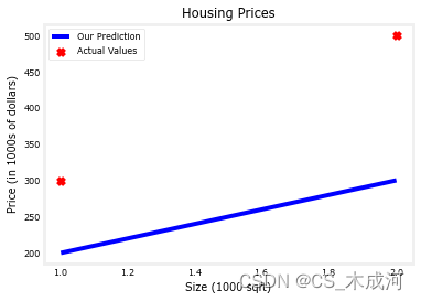
很明显， $w = 100$ 和 $b = 100$ 不会产生适合数据的直线。

根据学过的数学知识，可以容易求出 $w = 200$ 和 $b = 100$

5、预测

现在我们已经有了一个模型，可以用它来做出房屋价格的预测。来预测一下 1200 平方英尺的房子的价格。由于面积单位为 1000 平方英尺，所以 $x$ 是1.2。

w = 200                         
b = 100    
x_i = 1.2
cost_1200sqft = w * x_i + b    

print(f"${cost_1200sqft:.0f} thousand dollars")

输出的结果是：$340 thousand dollars

总结

线性回归建立一个特征和目标之间关系的模型
- 在上面的例子中，特征是房屋面积，目标是房价。
- 对于简单线性回归，模型有两个参数 $w$ 和 $b$ ，其值使用训练数据进行拟合。
- 一旦确定了模型的参数，该模型就可以用于对新数据进行预测。

附录

deeplearning.mplstyle 源码：

# see https://matplotlib.org/stable/tutorials/introductory/customizing.html
lines.linewidth: 4
lines.solid_capstyle: butt

legend.fancybox: true

# Verdana" for non-math text,
# Cambria Math

#Blue (Crayon-Aqua) 0096FF
#Dark Red C00000
#Orange (Apple Orange) FF9300
#Black 000000
#Magenta FF40FF
#Purple 7030A0

axes.prop_cycle: cycler('color', ['0096FF', 'FF9300', 'FF40FF', '7030A0', 'C00000'])
#axes.facecolor: f0f0f0 # grey
axes.facecolor: ffffff  # white
axes.labelsize: large
axes.axisbelow: true
axes.grid: False
axes.edgecolor: f0f0f0
axes.linewidth: 3.0
axes.titlesize: x-large

patch.edgecolor: f0f0f0
patch.linewidth: 0.5

svg.fonttype: path

grid.linestyle: -
grid.linewidth: 1.0
grid.color: cbcbcb

xtick.major.size: 0
xtick.minor.size: 0
ytick.major.size: 0
ytick.minor.size: 0

savefig.edgecolor: f0f0f0
savefig.facecolor: f0f0f0

#figure.subplot.left: 0.08
#figure.subplot.right: 0.95
#figure.subplot.bottom: 0.07

#figure.facecolor: f0f0f0  # grey
figure.facecolor: ffffff  # white

## ***************************************************************************
## * FONT                                                                    *
## ***************************************************************************
## The font properties used by `text.Text`.
## See https://matplotlib.org/api/font_manager_api.html for more information
## on font properties.  The 6 font properties used for font matching are
## given below with their default values.
##
## The font.family property can take either a concrete font name (not supported
## when rendering text with usetex), or one of the following five generic
## values:
##     - 'serif' (e.g., Times),
##     - 'sans-serif' (e.g., Helvetica),
##     - 'cursive' (e.g., Zapf-Chancery),
##     - 'fantasy' (e.g., Western), and
##     - 'monospace' (e.g., Courier).
## Each of these values has a corresponding default list of font names
## (font.serif, etc.); the first available font in the list is used.  Note that
## for font.serif, font.sans-serif, and font.monospace, the first element of
## the list (a DejaVu font) will always be used because DejaVu is shipped with
## Matplotlib and is thus guaranteed to be available; the other entries are
## left as examples of other possible values.
##
## The font.style property has three values: normal (or roman), italic
## or oblique.  The oblique style will be used for italic, if it is not
## present.
##
## The font.variant property has two values: normal or small-caps.  For
## TrueType fonts, which are scalable fonts, small-caps is equivalent
## to using a font size of 'smaller', or about 83%% of the current font
## size.
##
## The font.weight property has effectively 13 values: normal, bold,
## bolder, lighter, 100, 200, 300, ..., 900.  Normal is the same as
## 400, and bold is 700.  bolder and lighter are relative values with
## respect to the current weight.
##
## The font.stretch property has 11 values: ultra-condensed,
## extra-condensed, condensed, semi-condensed, normal, semi-expanded,
## expanded, extra-expanded, ultra-expanded, wider, and narrower.  This
## property is not currently implemented.
##
## The font.size property is the default font size for text, given in points.
## 10 pt is the standard value.
##
## Note that font.size controls default text sizes.  To configure
## special text sizes tick labels, axes, labels, title, etc., see the rc
## settings for axes and ticks.  Special text sizes can be defined
## relative to font.size, using the following values: xx-small, x-small,
## small, medium, large, x-large, xx-large, larger, or smaller


font.family:  sans-serif
font.style:   normal
font.variant: normal
font.weight:  normal
font.stretch: normal
font.size:    8.0

font.serif:      DejaVu Serif, Bitstream Vera Serif, Computer Modern Roman, New Century Schoolbook, Century Schoolbook L, Utopia, ITC Bookman, Bookman, Nimbus Roman No9 L, Times New Roman, Times, Palatino, Charter, serif
font.sans-serif: Verdana, DejaVu Sans, Bitstream Vera Sans, Computer Modern Sans Serif, Lucida Grande, Geneva, Lucid, Arial, Helvetica, Avant Garde, sans-serif
font.cursive:    Apple Chancery, Textile, Zapf Chancery, Sand, Script MT, Felipa, Comic Neue, Comic Sans MS, cursive
font.fantasy:    Chicago, Charcoal, Impact, Western, Humor Sans, xkcd, fantasy
font.monospace:  DejaVu Sans Mono, Bitstream Vera Sans Mono, Computer Modern Typewriter, Andale Mono, Nimbus Mono L, Courier New, Courier, Fixed, Terminal, monospace


## ***************************************************************************
## * TEXT                                                                    *
## ***************************************************************************
## The text properties used by `text.Text`.
## See https://matplotlib.org/api/artist_api.html#module-matplotlib.text
## for more information on text properties
#text.color: black