文章目录
- 实验要求
- 数据集定义
- 1 手写二维卷积
- 1.1 自定义卷积通道
- 1.2 自定义卷积层
- 1.3 添加卷积层导模块中
- 1.4 定义超参数
- 1.5 初始化模型、损失函数、优化器
- 1.6 定义模型训练和测试函数,输出训练集和测试集的损失和精确度
- 1.7 训练
- 1.8 loss及acc可视化
- 2 torch.nn 实现二维卷积
- 2.1 torch定义二维卷积
- 2.2 训练
- 2.3 loss及acc可视化
- 3 不同超参数的对比分析
- 3.1 不同lr
- 4 Alexnet网络
实验要求
- 手写二维卷积的实现,并在至少一个数据集上进行实验,从训练时间、预测精度、Loss变化等角度分析实验结果(最好使用图表展示)
- 使用torch.nn实现二维卷积,并在至少一个数据集上进行实验,从训练时间、预测精度、Loss变化等角度分析实验结果(最好使用图表展示)
- 不同的超参数的对比分析(包括卷积层数、卷积核大小、batchsize、lr等)选其中至少1-2个进行分析
- 选用PyTorch实现经典模型AlexNet并在至少一个数据集上进行试验分析
数据集定义
#导入相应的库
import torch
import numpy as np
import random
from matplotlib import pyplot as plt
import torch.utils.data as Data
from PIL import Image
import os
from torch import nn
import torch.optim as optim
from torch.nn import init
import torch.nn.functional as F
import time
import torchvision
from torchvision import transforms,datasets
from shutil import copy, rmtree
import json
/root/miniconda3/envs/pytorch12.1/lib/python3.8/site-packages/tqdm/auto.py:22: TqdmWarning: IProgress not found. Please update jupyter and ipywidgets. See https://ipywidgets.readthedocs.io/en/stable/user_install.html
  from .autonotebook import tqdm as notebook_tqdm
Duplicate key in file PosixPath('/root/miniconda3/envs/pytorch12.1/lib/python3.8/site-packages/matplotlib/mpl-data/matplotlibrc'), line 270 ('font.family : sans-serif')
定义一个函数用来生成相应的文件夹
def mk_file(file_path: str):
    if os.path.exists(file_path):
        # 如果文件夹存在,则先删除原文件夹在重新创建
        rmtree(file_path)
    os.makedirs(file_path)
定义划分数据集的函数split_data(),将数据集进行划分训练集和测试集
#定义函数划分数据集
def split_data():
    random.seed(0)
    # 将数据集中25%的数据划分到验证集中
    split_rate = 0.25

    # 指向你解压后的flower_photos文件夹
    cwd = os.getcwd()
    data_root = os.path.join(cwd, "data")
    origin_car_path = os.path.join(data_root, "vehcileClassificationDataset")
    assert os.path.exists(origin_car_path), "path '{}' does not exist.".format(origin_flower_path)

    car_class = [cla for cla in os.listdir(origin_car_path)
                    if os.path.isdir(os.path.join(origin_car_path, cla))]

    # 建立保存训练集的文件夹
    train_root = os.path.join(origin_car_path, "train")
    mk_file(train_root)
    for cla in car_class:
        # 建立每个类别对应的文件夹
        mk_file(os.path.join(train_root, cla))

    # 建立保存验证集的文件夹
    test_root = os.path.join(origin_car_path, "test")
    mk_file(test_root)
    for cla in car_class:
        # 建立每个类别对应的文件夹
        mk_file(os.path.join(test_root, cla))

    for cla in car_class:
        cla_path = os.path.join(origin_car_path, cla)
        images = os.listdir(cla_path)
        num = len(images)
        # 随机采样验证集的索引
        eval_index = random.sample(images, k=int(num*split_rate))
        for index, image in enumerate(images):
            if image in eval_index:
                # 将分配至验证集中的文件复制到相应目录
                image_path = os.path.join(cla_path, image)
                new_path = os.path.join(test_root, cla)
                copy(image_path, new_path)
            else:
                # 将分配至训练集中的文件复制到相应目录
                image_path = os.path.join(cla_path, image)
                new_path = os.path.join(train_root, cla)
                copy(image_path, new_path)
            print("\r[{}] processing [{}/{}]".format(cla, index+1, num), end="")  # processing bar
        print()

    print("processing done!")
split_data()
[bus] processing [219/219]
[car] processing [779/779]
[truck] processing [360/360]
processing done!
将划分好的数据集利用DataLoader进行迭代读取,ImageFolder是pytorch中通用的数据加载器,不同类别的车辆放在不同的文件夹,ImageFolder可以根据文件夹的名字进行相应的转化。这里定义一个batch size为128
device = torch.device("cuda:0" if torch.cuda.is_available() else "cpu")
print("using {} device.".format(device))

data_transform = {"train": transforms.Compose([transforms.Resize((64,64)),
                               transforms.RandomHorizontalFlip(),
                                transforms.ToTensor(),
                              transforms.Normalize((0.5,0.5,0.5),
                                                     (0.5,0.5,0.5))]),
          "test": transforms.Compose([transforms.Resize((64,64)),
                                      transforms.ToTensor(),
                              transforms.Normalize((0.5,0.5,0.5),
                                                    (0.5,0.5,0.5))])}

data_root =os.getcwd()
image_path = os.path.join(data_root,"data/vehcileClassificationDataset")
print(image_path)


train_dataset = datasets.ImageFolder(root=os.path.join(image_path,"train"),
                                     transform = data_transform["train"])

train_num = len(train_dataset)
print(train_num)

batch_size = 128

train_loader = torch.utils.data.DataLoader(train_dataset,
                                         batch_size = batch_size,
                                           shuffle = True,
                                           num_workers = 0)


test_dataset = datasets.ImageFolder(root=os.path.join(image_path,"test"),
                              transform = data_transform["test"])

test_num = len(test_dataset)
print(test_num)#val_num = 364
test_loader = torch.utils.data.DataLoader(test_dataset,
                                         batch_size = batch_size,
                                          shuffle=False,
                                           num_workers = 0)

print("using {} images for training, {} images for validation .".format(train_num,test_num))
using cuda:0 device.
/root/autodl-tmp/courses_deep/data/vehcileClassificationDataset
1019
338
using 1019 images for training, 338 images for validation .
1 手写二维卷积
1.1 自定义卷积通道
# 自定义单通道卷积
def corr2d(X,K):
    '''
    X:输入,shape (batch_size,H,W)
    K:卷积核,shape (k_h,k_w)
    '''
    batch_size,H,W = X.shape
    k_h,k_w = K.shape
    #初始化结果矩阵
    Y = torch.zeros((batch_size,H-k_h+1,W-k_w+1)).to(device)
    for i in range(Y.shape[1]):
        for j in range(Y.shape [2]):
            Y[:,i,j] = (X[:,i:i+k_h,j:j+k_w]* K).sum()
    return Y

#自定义多通道卷积
def corr2d_multi_in(X,K):
    '''
    输入X:维度(batch_size,C_in,H, W)
    卷积核K:维度(C_in,k_h,k_w)
    输出:维度(batch_size,H_out,W_out)
    '''
    #先计算第一通道
    res = corr2d(X[:,0,:,:], K[0,:,:])
    for i in range(1, X.shape[1]):
        #按通道相加
        res += corr2d(X[:,i,:,:], K[i,:,:])
    return res

#自定义多个多通道卷积
def corr2d_multi_in_out(X, K):
 # X: shape (batch_size,C_in,H,W)
 # K: shape (C_out,C_in,h,w)
 # Y: shape(batch_size,C_out,H_out,W_out)
    return torch.stack([corr2d_multi_in(X, k) for k in K],dim=1)
1.2 自定义卷积层
class MyConv2D(nn.Module):
    def __init__(self,in_channels, out_channels,kernel_size):
        super(MyConv2D,self).__init__()
        #初始化卷积层的2个参数:卷积核、偏差
       #isinstance判断类型
        if isinstance(kernel_size,int):
            kernel_size = (kernel_size,kernel_size)
            self.weight = nn.Parameter(torch.randn((out_channels, in_channels) + kernel_size)).to(device)
            self.bias = nn.Parameter(torch.randn(out_channels,1,1)).to(device)
    def forward(self,x):    #x:输入图片,维度(batch_size,C_in,H,W)
        return corr2d_multi_in_out(x,self.weight) + self.bias
1.3 添加卷积层导模块中
#添加自定义卷积层到模块中
class MyConvModule(nn.Module):
    def __init__(self):
        super(MyConvModule,self).__init__()
        #定义一层卷积层
        self.conv = nn.Sequential(
            MyConv2D(in_channels = 3,out_channels = 32,kernel_size = 3),
            nn.BatchNorm2d(32),
            # inplace-选择是否进行覆盖运算
            nn.ReLU(inplace=True))
        #输出层,将通道数变为分类数量
        self.fc = nn.Linear(32,num_classes)

    def forward(self,x):
        #图片经过一层卷积,输出维度变为(batch_size,C_out,H,W)
        out = self.conv(x)
        #使用平均池化层将图片的大小变为1x1,第二个参数为最后输出的长和宽(这里默认相等了)64-3/1 + 1 =62
        out = F.avg_pool2d(out,62)
        #将张量out从shape batchx32x1x1 变为 batch x32
        out = out.squeeze()
        #输入到全连接层将输出的维度变为3
        out = self.fc(out)
        return out
1.4 定义超参数
num_classes = 3
lr = 0.001
epochs = 5
1.5 初始化模型、损失函数、优化器
#初始化模型
net = MyConvModule().to(device)
#使用多元交叉熵损失函数
criterion = nn.CrossEntropyLoss()
#使用Adam优化器
optimizer = optim.Adam(net.parameters(),lr = lr)
1.6 定义模型训练和测试函数,输出训练集和测试集的损失和精确度
def train_epoch(net, data_loader, device):

    net.train() #指定当前为训练模式
    train_batch_num = len(data_loader) #记录共有多少个batch
    total_1oss = 0 #记录Loss
    correct = 0 #记录共有多少个样本被正确分类
    sample_num = 0 #记录样本总数

    #遍历每个batch进行训练
    for batch_idx, (data,target) in enumerate (data_loader):
        t1 = time.time()
        #将图片放入指定的device中
        data = data.to(device).float()
        #将图片标签放入指定的device中
        target = target.to(device).long()
        #将当前梯度清零
        optimizer.zero_grad()
        #使用模型计算出结果
        output = net(data)
        #计算损失
        loss = criterion(output, target.squeeze())
        #进行反向传播
        loss.backward()
        optimizer.step()
        #累加loss
        total_1oss += loss.item( )
        #找出每个样本值最大的idx,即代表预测此图片属于哪个类别
        prediction = torch.argmax(output, 1)
        #统计预测正确的类别数量
        correct += (prediction == target).sum().item()
        #累加当前的样本总数
        sample_num += len(prediction)
        #if batch_idx//5 ==0:
        t2 = time.time()
        print("processing:{}/{},消耗时间{}s".
                      format(batch_idx+1,len(data_loader),t2-t1))

    #计算平均oss与准确率
    loss = total_1oss / train_batch_num
    acc = correct / sample_num
    return loss, acc

def test_epoch(net, data_loader, device):
    net.eval() #指定当前模式为测试模式
    test_batch_num = len(data_loader)
    total_loss = 0
    correct = 0
    sample_num = 0
    #指定不进行梯度变化
    with torch.no_grad():
        for batch_idx, (data, target) in enumerate(data_loader):
            data = data.to(device).float()
            target = target.to(device).long()
            output = net(data)
            loss = criterion(output, target)
            total_loss += loss.item( )
            prediction = torch.argmax(output, 1)
            correct += (prediction == target).sum().item()
            sample_num += len(prediction)
    loss = total_loss / test_batch_num
    acc = correct / sample_num
    return loss,acc
1.7 训练
#### 存储每一个epoch的loss与acc的变化,便于后面可视化
train_loss_list = []
train_acc_list = []
test_loss_list = []
test_acc_list = []
time_list = []
timestart = time.time()
#进行训练
for epoch in range(epochs):
    #每一个epoch的开始时间
    epochstart = time.time()

    #在训练集上训练
    train_loss, train_acc = train_epoch(net,data_loader=train_loader, device=device )
    #在测试集上验证
    test_loss, test_acc = test_epoch(net,data_loader=test_loader, device=device)

    #每一个epoch的结束时间
    elapsed = (time.time() - epochstart)
    #保存各个指际
    train_loss_list.append(train_loss)
    train_acc_list.append(train_acc )
    test_loss_list.append(test_loss)
    test_acc_list.append(test_acc)
    time_list.append(elapsed)
    print('epoch %d, train_loss %.6f,test_loss %.6f,train_acc %.6f,test_acc %.6f,Time used %.6fs'%(epoch+1, train_loss,test_loss,train_acc,test_acc,elapsed))
#计算总时间
timesum = (time.time() - timestart)
print('The total time is %fs',timesum)
processing:1/8,消耗时间49.534741163253784s
processing:2/8,消耗时间53.82337474822998s
processing:3/8,消耗时间54.79615521430969s
processing:4/8,消耗时间54.47013306617737s
processing:5/8,消耗时间54.499276638031006s
processing:6/8,消耗时间54.50710964202881s
processing:7/8,消耗时间53.65488290786743s
processing:8/8,消耗时间53.24664235115051s
epoch 1, train_loss 1.136734,test_loss 1.105827,train_acc 0.264966,test_acc 0.266272,Time used 471.139387s
processing:1/8,消耗时间48.97239923477173s
processing:2/8,消耗时间52.72454595565796s
processing:3/8,消耗时间53.08940005302429s
processing:4/8,消耗时间53.7891743183136s
processing:5/8,消耗时间53.07097554206848s
processing:6/8,消耗时间53.59272122383118s
processing:7/8,消耗时间53.85381197929382s
processing:8/8,消耗时间54.998770236968994s
epoch 2, train_loss 1.077828,test_loss 1.038692,train_acc 0.391560,test_acc 0.573964,Time used 466.846851s
processing:1/8,消耗时间49.87800121307373s
processing:2/8,消耗时间50.94171380996704s
processing:3/8,消耗时间51.578328371047974s
processing:4/8,消耗时间52.10942506790161s
processing:5/8,消耗时间53.03168201446533s
processing:6/8,消耗时间53.60364890098572s
processing:7/8,消耗时间53.400307416915894s
processing:8/8,消耗时间53.074254274368286s
epoch 3, train_loss 1.035702,test_loss 0.995151,train_acc 0.574092,test_acc 0.573964,Time used 460.014597s
processing:1/8,消耗时间49.56705284118652s
processing:2/8,消耗时间50.62346339225769s
processing:3/8,消耗时间51.27069616317749s
processing:4/8,消耗时间52.584522008895874s
processing:5/8,消耗时间53.778876304626465s
processing:6/8,消耗时间54.50534129142761s
processing:7/8,消耗时间54.09490990638733s
processing:8/8,消耗时间53.962727785110474s
epoch 4, train_loss 1.003914,test_loss 0.967035,train_acc 0.574092,test_acc 0.573964,Time used 462.696877s
processing:1/8,消耗时间49.09861469268799s
processing:2/8,消耗时间50.945659160614014s
processing:3/8,消耗时间51.85160732269287s
processing:4/8,消耗时间52.68898820877075s
processing:5/8,消耗时间52.44323921203613s
processing:6/8,消耗时间53.98334002494812s
processing:7/8,消耗时间53.38289451599121s
processing:8/8,消耗时间53.83491349220276s
epoch 5, train_loss 0.984345,test_loss 0.949488,train_acc 0.574092,test_acc 0.573964,Time used 460.776392s
The total time is %fs 2321.475680589676
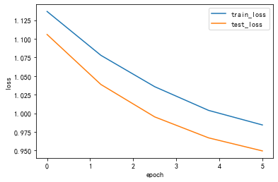
1.8 loss及acc可视化
def Draw_Curve(*args,xlabel = "epoch",ylabel = "loss"):#
for i in args:
x = np.linspace(0,len(i[0]),len(i[0]))
plt.plot(x,i[0],label=i[1],linewidth=1.5)
plt.xlabel(xlabel)
plt.ylabel(ylabel)
plt.legend()
plt.show()
Draw_Curve([train_acc_list,"train_acc"],[test_acc_list,"test_acc"],ylabel = "acc")
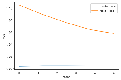
Draw_Curve([train_loss_list,"train_loss"],[test_loss_list,"test_loss"])

2 torch.nn 实现二维卷积
与手写二维卷积除了模型定义和不同外,其他均相同
2.1 torch定义二维卷积
   #pytorch封装卷积层
class ConvModule(nn.Module):
    def __init__(self):
        super(ConvModule,self).__init__()
        #定义三层卷积层
        self.conv = nn.Sequential(
            #第一层
            nn.Conv2d(in_channels = 3,out_channels = 32,
                         kernel_size = 3 , stride = 1,padding=0),
            nn.BatchNorm2d(32),
            # inplace-选择是否进行覆盖运算
            nn.ReLU(inplace=True),
            #第二层
            nn.Conv2d(in_channels = 32,out_channels = 64,
                         kernel_size = 3 , stride = 1,padding=0),
            nn.BatchNorm2d(64),
            # inplace-选择是否进行覆盖运算
            nn.ReLU(inplace=True),
            #第三层
            nn.Conv2d(in_channels = 64,out_channels = 128,
                        kernel_size = 3 , stride = 1,padding=0),
            nn.BatchNorm2d(128),
            # inplace-选择是否进行覆盖运算
            nn.ReLU(inplace=True)
        )
        #输出层,将通道数变为分类数量
        self.fc = nn.Linear(128,num_classes)

    def forward(self,x):
        #图片经过三层卷积,输出维度变为(batch_size,C_out,H,W)
        out = self.conv(x)
        #使用平均池化层将图片的大小变为1x1,第二个参数为最后输出的长和宽(这里默认相等了)(64-3)/1 + 1 =62  (62-3)/1+1 =60 (60-3)/1+1 =58
        out = F.avg_pool2d(out,58)
        #将张量out从shape batchx128x1x1 变为 batch x128
        out = out.squeeze()
        #输入到全连接层将输出的维度变为3
        out = self.fc(out)
        return out
2.2 训练
# 更换为ConvModule
net = ConvModule().to(device)

#### 存储每一个epoch的loss与acc的变化,便于后面可视化
train_loss_list = []
train_acc_list = []
test_loss_list = []
test_acc_list = []
time_list = []
timestart = time.time()
#进行训练
for epoch in range(epochs):
    #每一个epoch的开始时间
    epochstart = time.time()

    #在训练集上训练
    train_loss, train_acc = train_epoch(net,data_loader=train_loader, device=device )
    #在测试集上验证
    test_loss, test_acc = test_epoch(net,data_loader=test_loader, device=device)

    #每一个epoch的结束时间
    elapsed = (time.time() - epochstart)
    #保存各个指际
    train_loss_list.append(train_loss)
    train_acc_list.append(train_acc )
    test_loss_list.append(test_loss)
    test_acc_list.append(test_acc)
    time_list.append(elapsed)
    print('epoch %d, train_loss %.6f,test_loss %.6f,train_acc %.6f,test_acc %.6f,Time used %.6fs'%(epoch+1, train_loss,test_loss,train_acc,test_acc,elapsed))
#计算总时间
timesum = (time.time() - timestart)
print('The total time is %fs',timesum)
processing:1/8,消耗时间1.384758710861206s
processing:2/8,消耗时间0.025571107864379883s
processing:3/8,消耗时间0.02555680274963379s
processing:4/8,消耗时间0.025563478469848633s
processing:5/8,消耗时间0.025562286376953125s
processing:6/8,消耗时间0.025719642639160156s
processing:7/8,消耗时间0.025638103485107422s
processing:8/8,消耗时间0.02569437026977539s
epoch 1, train_loss 1.134971,test_loss 1.104183,train_acc 0.131501,test_acc 0.133136,Time used 2.488544s
processing:1/8,消耗时间0.02553415298461914s
processing:2/8,消耗时间0.025570392608642578s
processing:3/8,消耗时间0.025498628616333008s
processing:4/8,消耗时间0.025622844696044922s
processing:5/8,消耗时间0.025777101516723633s
processing:6/8,消耗时间0.0256195068359375s
processing:7/8,消耗时间0.02576303482055664s
processing:8/8,消耗时间0.02545619010925293s
epoch 2, train_loss 1.134713,test_loss 1.102343,train_acc 0.123651,test_acc 0.239645,Time used 1.160389s
processing:1/8,消耗时间0.025580883026123047s
processing:2/8,消耗时间0.025583267211914062s
processing:3/8,消耗时间0.025578737258911133s
processing:4/8,消耗时间0.025538921356201172s
processing:5/8,消耗时间0.025668621063232422s
processing:6/8,消耗时间0.02561044692993164s
processing:7/8,消耗时间0.02561807632446289s
processing:8/8,消耗时间0.02550649642944336s
epoch 3, train_loss 1.134326,test_loss 1.105134,train_acc 0.129539,test_acc 0.186391,Time used 1.124050s
processing:1/8,消耗时间0.025658130645751953s
processing:2/8,消耗时间0.025626659393310547s
processing:3/8,消耗时间0.02562260627746582s
processing:4/8,消耗时间0.02557849884033203s
processing:5/8,消耗时间0.025677204132080078s
processing:6/8,消耗时间0.025617122650146484s
processing:7/8,消耗时间0.02563309669494629s
processing:8/8,消耗时间0.025460243225097656s
epoch 4, train_loss 1.134662,test_loss 1.111777,train_acc 0.127576,test_acc 0.115385,Time used 1.105919s
processing:1/8,消耗时间0.025597333908081055s
processing:2/8,消耗时间0.025560379028320312s
processing:3/8,消耗时间0.025528430938720703s
processing:4/8,消耗时间0.025620698928833008s
processing:5/8,消耗时间0.025687694549560547s
processing:6/8,消耗时间0.025610685348510742s
processing:7/8,消耗时间0.02558135986328125s
processing:8/8,消耗时间0.025484323501586914s
epoch 5, train_loss 1.134296,test_loss 1.117432,train_acc 0.131501,test_acc 0.106509,Time used 1.103042s
The total time is %fs 6.982609033584595
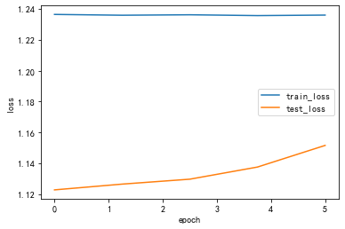
2.3 loss及acc可视化
Draw_Curve([train_acc_list,"train_acc"],[test_acc_list,"test_acc"],ylabel = "acc")
Draw_Curve([train_loss_list,"train_loss"],[test_loss_list,"test_loss"])


3 不同超参数的对比分析
- 学习率lr对模型的影响,选择学习率lr = 0.1、0.01、0.01
- batchsize对模型的影响,设置batch_size = 64、128
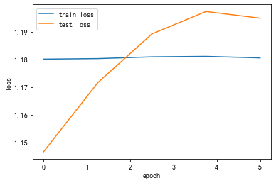
3.1 不同lr
lr_list = [0.1,0.01,0.001]
for lr in lr_list :
    print("lr:",lr)
    optimizer = optim.Adam(net.parameters(),lr = lr)

    # 更换为ConvModule
    net = ConvModule().to(device)

    #### 存储每一个epoch的loss与acc的变化,便于后面可视化
    train_loss_list = []
    train_acc_list = []
    test_loss_list = []
    test_acc_list = []
    time_list = []
    timestart = time.time()
    #进行训练
    for epoch in range(epochs):
        #每一个epoch的开始时间
        epochstart = time.time()

        #在训练集上训练
        train_loss, train_acc = train_epoch(net,data_loader=train_loader, device=device )
        #在测试集上验证
        test_loss, test_acc = test_epoch(net,data_loader=test_loader, device=device)

        #每一个epoch的结束时间
        elapsed = (time.time() - epochstart)
        #保存各个指际
        train_loss_list.append(train_loss)
        train_acc_list.append(train_acc )
        test_loss_list.append(test_loss)
        test_acc_list.append(test_acc)
        time_list.append(elapsed)
        print('epoch %d, train_loss %.6f,test_loss %.6f,train_acc %.6f,test_acc %.6f,Time used %.6fs'%(epoch+1, train_loss,test_loss,train_acc,test_acc,elapsed))
    Draw_Curve([train_acc_list,"train_acc"],[test_acc_list,"test_acc"],ylabel = "acc")
    Draw_Curve([train_loss_list,"train_loss"],[test_loss_list,"test_loss"])
lr: 0.1
processing:1/8,消耗时间0.025880813598632812s
processing:2/8,消耗时间0.02591729164123535s
processing:3/8,消耗时间0.025969743728637695s
processing:4/8,消耗时间0.02597641944885254s
processing:5/8,消耗时间0.0259091854095459s
processing:6/8,消耗时间0.025940418243408203s
processing:7/8,消耗时间0.02597665786743164s
processing:8/8,消耗时间0.025816917419433594s
epoch 1, train_loss 1.236414,test_loss 1.122834,train_acc 0.312071,test_acc 0.266272,Time used 1.150748s
processing:1/8,消耗时间0.02601909637451172s
processing:2/8,消耗时间0.026076078414916992s
processing:3/8,消耗时间0.02595829963684082s
processing:4/8,消耗时间0.02597641944885254s
processing:5/8,消耗时间0.025915145874023438s
processing:6/8,消耗时间0.02601909637451172s
processing:7/8,消耗时间0.025966167449951172s
processing:8/8,消耗时间0.025896072387695312s
epoch 2, train_loss 1.235889,test_loss 1.126564,train_acc 0.307164,test_acc 0.266272,Time used 1.130118s
processing:1/8,消耗时间0.025966405868530273s
processing:2/8,消耗时间0.026023387908935547s
processing:3/8,消耗时间0.02602076530456543s
processing:4/8,消耗时间0.025955677032470703s
processing:5/8,消耗时间0.026730775833129883s
processing:6/8,消耗时间0.02618265151977539s
processing:7/8,消耗时间0.025946378707885742s
processing:8/8,消耗时间0.025950908660888672s
epoch 3, train_loss 1.236183,test_loss 1.129753,train_acc 0.311089,test_acc 0.266272,Time used 1.138533s
processing:1/8,消耗时间0.0259554386138916s
processing:2/8,消耗时间0.02595067024230957s
processing:3/8,消耗时间0.025972843170166016s
processing:4/8,消耗时间0.025902509689331055s
processing:5/8,消耗时间0.025956392288208008s
processing:6/8,消耗时间0.02594304084777832s
processing:7/8,消耗时间0.02598118782043457s
processing:8/8,消耗时间0.025868892669677734s
epoch 4, train_loss 1.235654,test_loss 1.137612,train_acc 0.309127,test_acc 0.263314,Time used 1.147009s
processing:1/8,消耗时间0.02599787712097168s
processing:2/8,消耗时间0.025910615921020508s
processing:3/8,消耗时间0.025928497314453125s
processing:4/8,消耗时间0.025904178619384766s
processing:5/8,消耗时间0.025990724563598633s
processing:6/8,消耗时间0.02588057518005371s
processing:7/8,消耗时间0.026009321212768555s
processing:8/8,消耗时间0.02586531639099121s
epoch 5, train_loss 1.235978,test_loss 1.151615,train_acc 0.307164,test_acc 0.272189,Time used 1.136342s

lr: 0.01
processing:1/8,消耗时间0.02597332000732422s
processing:2/8,消耗时间0.025891780853271484s
processing:3/8,消耗时间0.0260159969329834s
processing:4/8,消耗时间0.025948286056518555s
processing:5/8,消耗时间0.026835918426513672s
processing:6/8,消耗时间0.026047945022583008s
processing:7/8,消耗时间0.02601790428161621s
processing:8/8,消耗时间0.0258333683013916s
epoch 1, train_loss 1.180047,test_loss 1.146577,train_acc 0.128557,test_acc 0.159763,Time used 1.166165s
processing:1/8,消耗时间0.025972843170166016s
processing:2/8,消耗时间0.02600264549255371s
processing:3/8,消耗时间0.025959253311157227s
processing:4/8,消耗时间0.025983333587646484s
processing:5/8,消耗时间0.026042699813842773s
processing:6/8,消耗时间0.02595233917236328s
processing:7/8,消耗时间0.025896310806274414s
processing:8/8,消耗时间0.025844335556030273s
epoch 2, train_loss 1.180246,test_loss 1.171511,train_acc 0.134446,test_acc 0.159763,Time used 1.122087s
processing:1/8,消耗时间0.0258941650390625s
processing:2/8,消耗时间0.025923728942871094s
processing:3/8,消耗时间0.02590012550354004s
processing:4/8,消耗时间0.026006698608398438s
processing:5/8,消耗时间0.025960922241210938s
processing:6/8,消耗时间0.02593088150024414s
processing:7/8,消耗时间0.025939226150512695s
processing:8/8,消耗时间0.025836944580078125s
epoch 3, train_loss 1.180876,test_loss 1.189146,train_acc 0.127576,test_acc 0.159763,Time used 1.112899s
processing:1/8,消耗时间0.025928497314453125s
processing:2/8,消耗时间0.025928974151611328s
processing:3/8,消耗时间0.025905132293701172s
processing:4/8,消耗时间0.02616095542907715s
processing:5/8,消耗时间0.02619624137878418s
processing:6/8,消耗时间0.025908946990966797s
processing:7/8,消耗时间0.02593541145324707s
processing:8/8,消耗时间0.025844812393188477s
epoch 4, train_loss 1.181045,test_loss 1.197265,train_acc 0.124632,test_acc 0.159763,Time used 1.130010s
processing:1/8,消耗时间0.025942325592041016s
processing:2/8,消耗时间0.02595806121826172s
processing:3/8,消耗时间0.025911331176757812s
processing:4/8,消耗时间0.026000499725341797s
processing:5/8,消耗时间0.026007890701293945s
processing:6/8,消耗时间0.025979042053222656s
processing:7/8,消耗时间0.02596426010131836s
processing:8/8,消耗时间0.025872468948364258s
epoch 5, train_loss 1.180506,test_loss 1.194845,train_acc 0.130520,test_acc 0.127219,Time used 1.125265s

lr: 0.001
processing:1/8,消耗时间0.025917768478393555s
processing:2/8,消耗时间0.02601337432861328s
processing:3/8,消耗时间0.02601933479309082s
processing:4/8,消耗时间0.025936603546142578s
processing:5/8,消耗时间0.025965213775634766s
processing:6/8,消耗时间0.025942087173461914s
processing:7/8,消耗时间0.025992393493652344s
processing:8/8,消耗时间0.025847673416137695s
epoch 1, train_loss 1.003024,test_loss 1.104485,train_acc 0.574092,test_acc 0.177515,Time used 1.128456s
processing:1/8,消耗时间0.025956392288208008s
processing:2/8,消耗时间0.026005983352661133s
processing:3/8,消耗时间0.025966167449951172s
processing:4/8,消耗时间0.0259397029876709s
processing:5/8,消耗时间0.025922298431396484s
processing:6/8,消耗时间0.025957107543945312s
processing:7/8,消耗时间0.02590632438659668s
processing:8/8,消耗时间0.02581644058227539s
epoch 2, train_loss 1.003732,test_loss 1.088773,train_acc 0.574092,test_acc 0.573964,Time used 1.124280s
processing:1/8,消耗时间0.02595043182373047s
processing:2/8,消耗时间0.026049375534057617s
processing:3/8,消耗时间0.02598428726196289s
processing:4/8,消耗时间0.026129961013793945s
processing:5/8,消耗时间0.02595376968383789s
processing:6/8,消耗时间0.02595376968383789s
processing:7/8,消耗时间0.02597832679748535s
processing:8/8,消耗时间0.025784730911254883s
epoch 3, train_loss 1.003739,test_loss 1.075143,train_acc 0.574092,test_acc 0.573964,Time used 1.123431s
processing:1/8,消耗时间0.026008129119873047s
processing:2/8,消耗时间0.0260159969329834s
processing:3/8,消耗时间0.025996923446655273s
processing:4/8,消耗时间0.025960683822631836s
processing:5/8,消耗时间0.02593994140625s
processing:6/8,消耗时间0.026180744171142578s
processing:7/8,消耗时间0.025992393493652344s
processing:8/8,消耗时间0.025855541229248047s
epoch 4, train_loss 1.003592,test_loss 1.063867,train_acc 0.574092,test_acc 0.573964,Time used 1.121493s
processing:1/8,消耗时间0.026531219482421875s
processing:2/8,消耗时间0.02593708038330078s
processing:3/8,消耗时间0.0260317325592041s
processing:4/8,消耗时间0.025905370712280273s
processing:5/8,消耗时间0.02595996856689453s
processing:6/8,消耗时间0.026064395904541016s
processing:7/8,消耗时间0.02595973014831543s
processing:8/8,消耗时间0.02584242820739746s
epoch 5, train_loss 1.003357,test_loss 1.057218,train_acc 0.574092,test_acc 0.573964,Time used 1.131697s

4 Alexnet网络
由于输入的图像为64×64,如果按照原始的Alax网络的参数进行定义网络,第一个卷积层的卷积核尺寸为11×11,步长stride为4,导致卷积过后的一些图像尺寸过小,丢失了图像特征,影响模型的精度。因此,本次实验,根据实验数据集的图像特点,对Alexnet网络的特征提取部分参数进行了修改
class AlexNet(nn.Module):
    def __init__(self,num_classes = 1000,init_weights = False):
        super(AlexNet,self).__init__()
        self.features = nn.Sequential(#输入64×64×3
            nn.Conv2d(3,48,kernel_size=3,stride=1,padding=1),#64,64,48
            nn.ReLU(inplace=True),
            nn.MaxPool2d(kernel_size=2,stride=2),#32,32,48

            nn.Conv2d(48,128,kernel_size=3,padding=1),#32,32,128
            nn.ReLU(inplace=True),
            nn.MaxPool2d(kernel_size=2,stride=2),#16,16,128

            nn.Conv2d(128,192,kernel_size=3,padding=1),#16,16,192
            nn.ReLU(inplace=True),

            nn.Conv2d(192,192,kernel_size=3,stride=2,padding=1),#8,8,192
            nn.ReLU(inplace=True),

            nn.Conv2d(192,128,kernel_size=3,padding=1),#8,8,128
            nn.ReLU(inplace=True),
            nn.MaxPool2d(kernel_size=2,stride=2),#4,4,128
        )
        self.classifier = nn.Sequential(
            nn.Dropout(p=0.5),
            nn.Linear(128*4*4,2048),
            nn.ReLU(inplace=True),
            nn.Dropout(p=0.5),
            nn.Linear(2048,2048),
            nn.ReLU(inplace=True),
            nn.Linear(2048,num_classes),
        )
        if init_weights:
            self._initialize_weights()

    def forward(self,x):
        x = self.features(x)
        x = torch.flatten(x,start_dim=1)
        x = self.classifier(x)
        return x


![[基因遗传算法]进阶之四:实践VRPTW](https://img-blog.csdnimg.cn/6f83890a67dd4741ab42695a5fa38679.png)