📋📋📋本文目录如下:🎁🎁🎁
目录
💥1 概述
📚2 运行结果
2.1 算例1
2.2 算例2
2.3 算例3
🎉3 参考文献
🌈4 Matlab代码、数据、文章
💥1 概述
摘要:
空气压缩机系统约占美国和欧盟工业用电量的10%。由于许多研究已经证明了使用人工神经网络进行空压机性能预测的有效性,因此仍然需要预测空压机的电气负荷曲线。本研究的目的是预测压缩空气系统的电气负载曲线,这对于行业从业者和软件提供商开发更好的负载管理和前瞻调度程序的实践和工具很有价值。采用两层前馈神经网络和长短期记忆两种人工神经网络对空压机的电气负荷进行预测。对具有三种不同控制机构的压缩机进行了评估,总共进行了 11,874 次观察。使用样本外数据集和 5 倍交叉验证对预测进行了验证。模型产生的平均决定系数值为0.24-0.94,平均均方根误差为0.05 kW - 5.83 kW,平均绝对比例误差为0.20 - 1.33。结果表明,两种人工神经网络对使用变速驱动的压缩机(平均R2 = 0.8且无中殿预测)均有较好的结果,只有长短期记忆模型对使用开/关控制的压缩机给出了可接受的结果(平均R2 = 0.82且无中殿预测),而对装卸式空压机(构成中殿预测的模型)没有获得满意的结果。
原文摘要:
Air compressor systems are responsible for approximately 10% of the electricity consumed in United States and European Union industry. As many researches have proven the effectiveness of using Artificial Neural Network in air compressor performance prediction, there is still a need to forecast the air compressor electrical load profile. The objective of this study is to predict compressed air systems' electrical load profile, which is valuable to industry practitioners as well as software providers in developing better practice and tools for load management and look-ahead scheduling programs. Two artificial neural networks, Two-Layer Feed-Forward Neural Network and Long Short-Term Memory were used to predict an air compressors electrical load. Compressors with three different control mechanisms are evaluated with a total number of 11,874 observations. The forecasts were validated using out-of-sample datasets with 5-fold cross-validation. Models produced average coefficient of determination values from 0.24 to 0.94, average root-mean-square errors from 0.05 kW - 5.83 kW, and mean absolute scaled errors from 0.20 to 1.33. The results indicate that both artificial neural networks yield good results for compressors using variable speed drive (average R2 = 0.8 and no naïve forecasting), only the long short-term memory model gives acceptable results for compressors using on/off control (average R2 = 0.82 and no naïve forecasting), and no satisfactory results are obtained for load/unload type air compressors (models constituting naïve forecasting).
📚2 运行结果
2.1 算例1
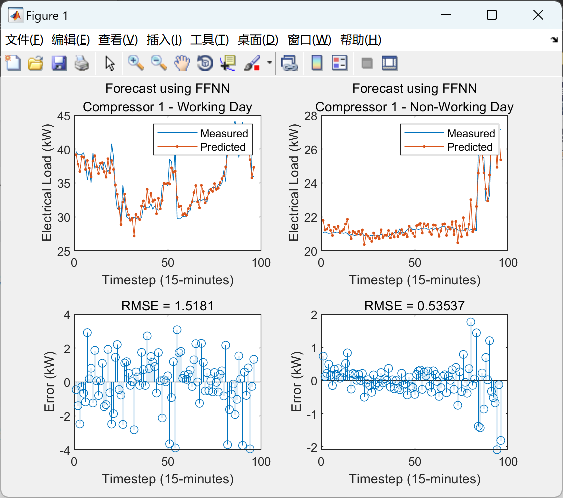
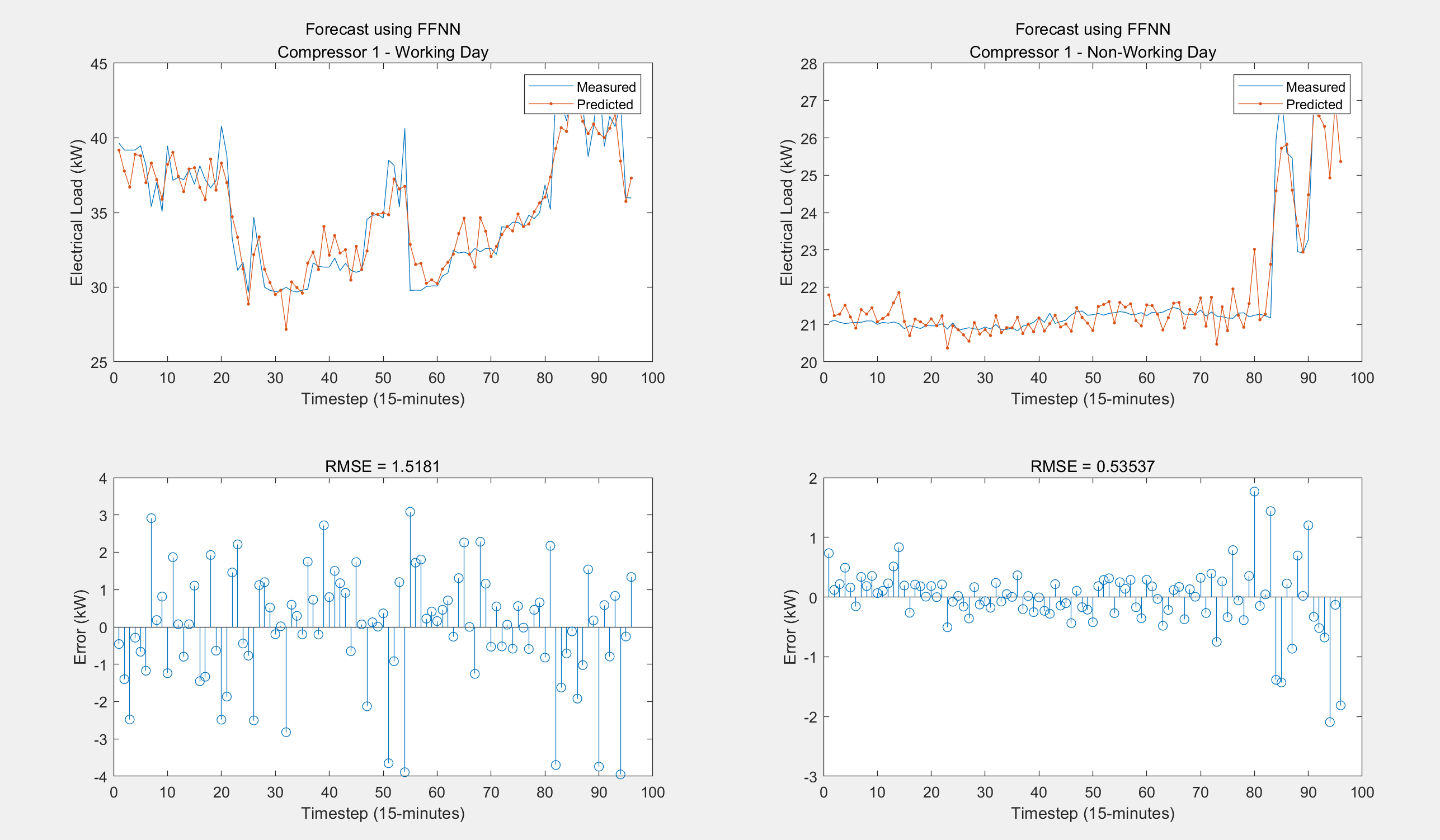
2.2 算例2
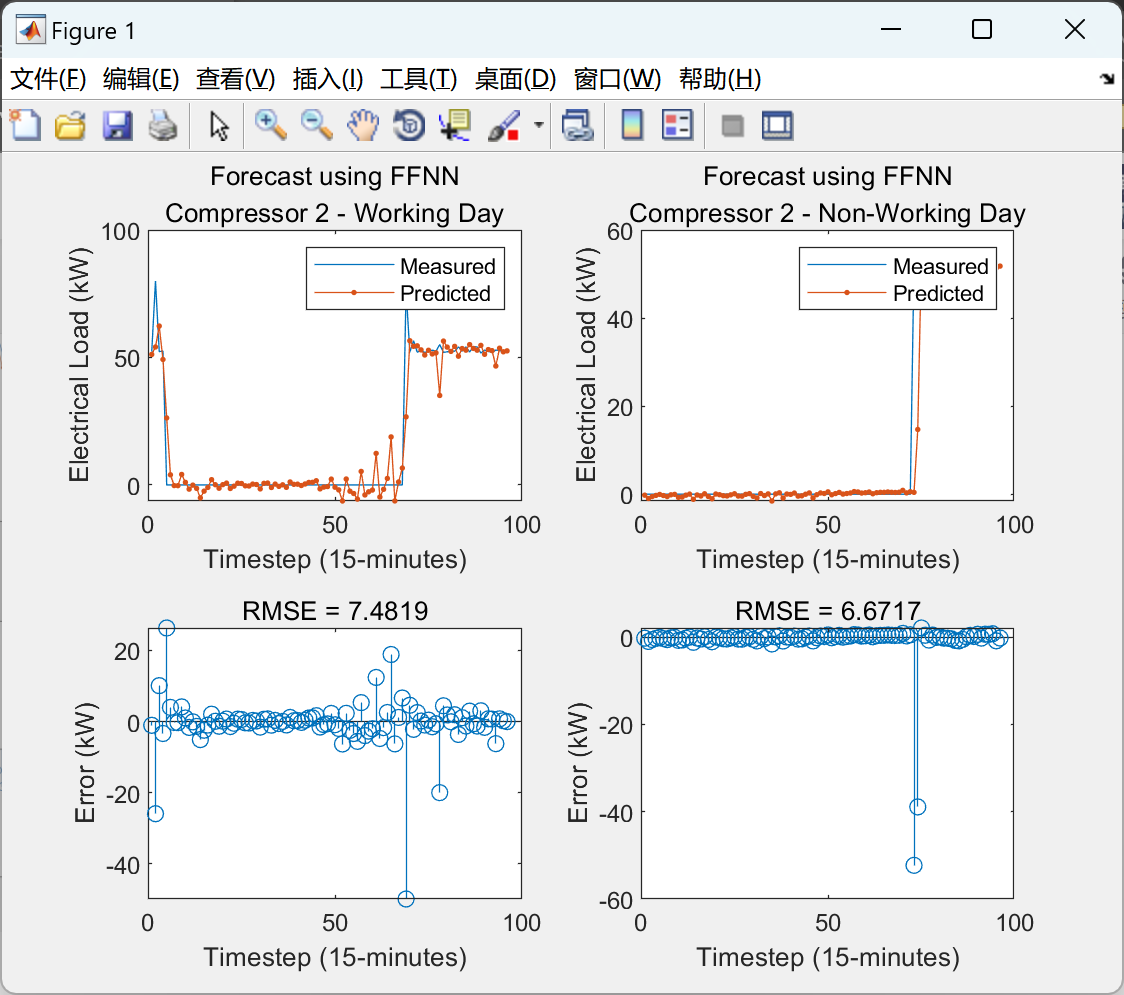
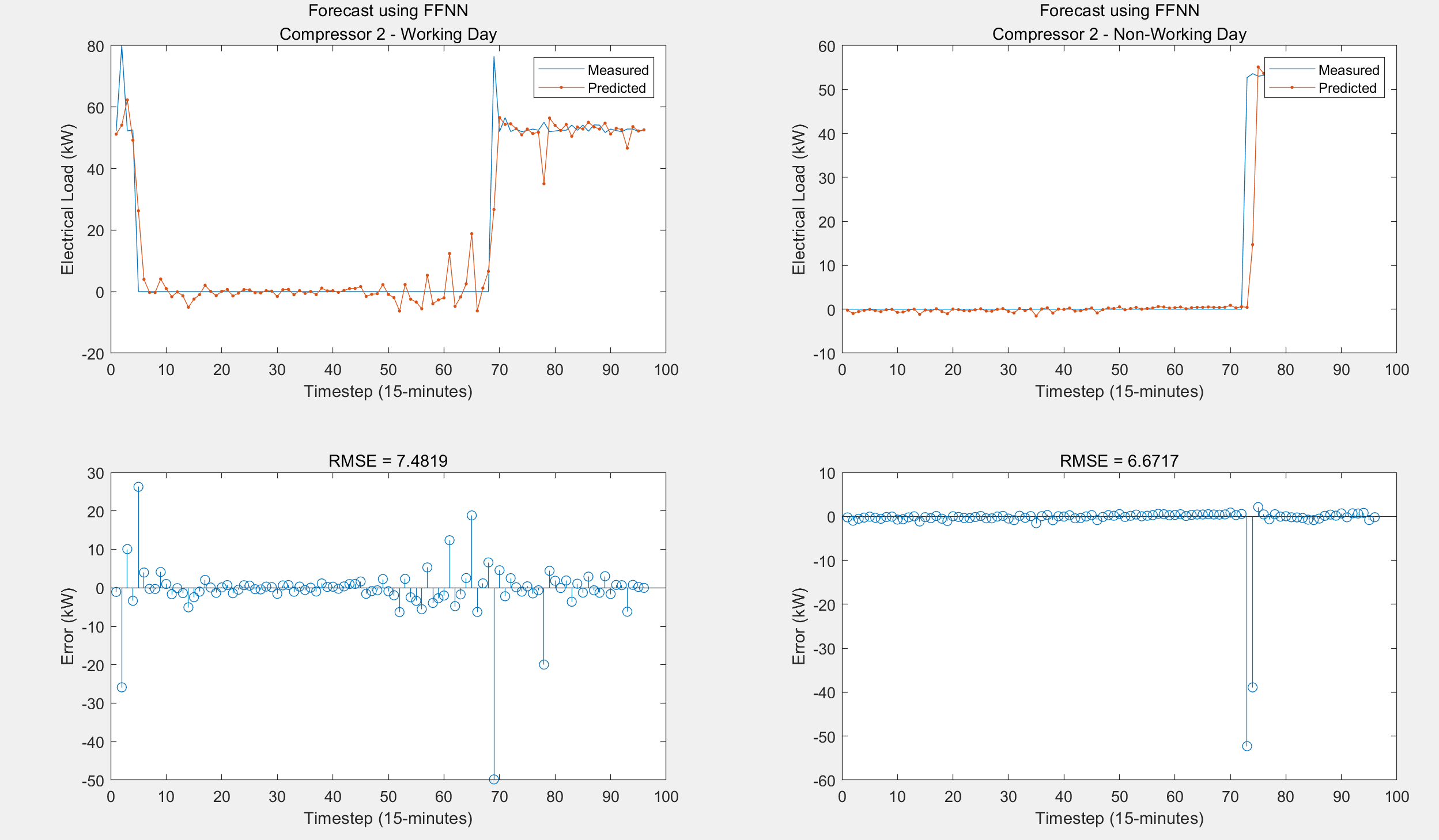
2.3 算例3
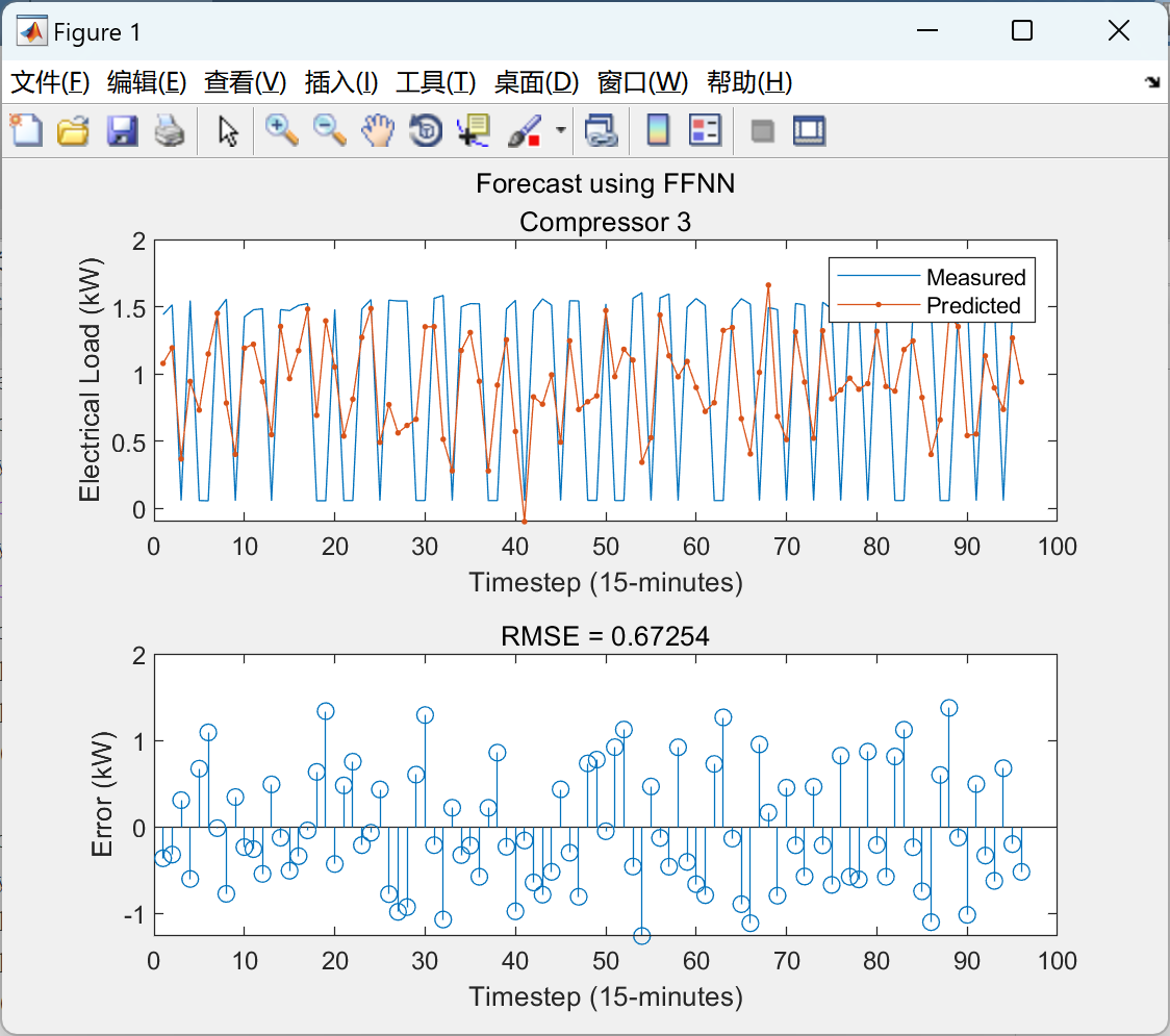
部分代码:
RMSE = sqrt(mean((y - yhat).^2)); % calculate root mean squared error
MASE = mean(abs(y-yhat))/(mean(abs(y(2:end)-y(1:end-1)))); % calculate mean absolute scaled error
mdl = fitlm(y,yhat);
R2 = mdl.Rsquared.Ordinary; % get R2 between observed and predicited
T = table (RMSE,MASE, R2,'RowNames',{'Working Days'}); % construct output table
T.Properties.DimensionNames{1} = 'Mode';
figure
subplot(2,1,1)
plot(y)
hold on
plot(yhat,'.-')
hold off
legend(["Measured" "Predicted"])
xlabel("Timestep (15-minutes)")
ylabel("Electrical Load (kW)")
title(["Forecast using FFNN";"Compressor 3"])
subplot(2,1,2)
stem(yhat - y)
xlabel("Timestep (15-minutes)")
ylabel("Error (kW)")
title("RMSE = " + RMSE)
🎉3 参考文献
部分理论来源于网络,如有侵权请联系删除。


