文章目录
- 说明
- Day58 符号型数据的 NB 算法
- 1.基础理论知识
- 1.1 条件概率
- 1.2 独立性假设
- 1.3 Laplacian 平滑
- 2. 符号型数据的预测算法跟踪
- 2.1 testNominal()方法
- 2.1.1 NaiveBayes 构造函数
- 2.1.2 calculateClassDistribution()
- 2.1.3 calculateConditionalProbabilities()方法
- 2.1.4 classify()方法
- 2.1.5 computeAccuracy() 计算精确性
- Day59 数值型数据的 NB 算法
- 1.基础理论知识
- 1.1 数值型和符号型NB 对比
- 1.2高斯分布(正态分布)
- 2.符号型数据的预测算法跟踪
- 2.1 testNumerical()方法
- 2.1.1 构造方法NaiveBayes
- 2.1.2 calculateClassDistribution()
- 2.1.3 calculateGausssianParameters()方法
- 2.1.4 classify()方法
说明
闵老师的文章链接: 日撸 Java 三百行(总述)_minfanphd的博客-CSDN博客
自己也把手敲的代码放在了github上维护:https://github.com/fulisha-ok/sampledata
Day58 符号型数据的 NB 算法
1.基础理论知识
(对老师这篇文章的翻译,以方便自己的理解)
1.1 条件概率
在给定某个条件下,事件发生的概率。它表示为 P(A|B),表示在事件 B 发生的条件下事件 A 发生的概率。
P(AB) 表示事件 A和B同时发生的概率;
p
(
A
∣
B
)
=
p
(
A
B
)
p
(
B
)
=
p
(
B
∣
A
)
∗
p
(
A
)
p
(
B
)
p(A|B) = \frac{p(AB)}{p(B)} = \frac{p(B|A)*p(A)}{p(B)}
p(A∣B)=p(B)p(AB)=p(B)p(B∣A)∗p(A)
1.2 独立性假设
假设特征之间是相互独立的,在计算概率时,我们可以假设每个特征的出现与其他特征无关,这样可以简化计算过程(虽然这个假设在现实中并不总是成立)
-
在x发生的条件下Di发生的概率,且假设各个特征之间是相互独立的(直接可以展开连乘)。
x 条件组合,如outlook=sunny∧temperature=hot; Di 表示一个事件, 如: play = No不出去玩
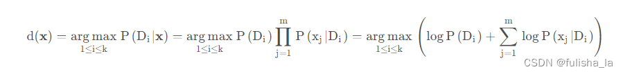
p ( D i ∣ x ) = p ( x D i ) p ( x ) = p ( D i ) p ( x ∣ D i ) p ( x ) = p ( D i ) ∏ j = 1 m p ( x j ∣ D i ) p ( x ) p(D_{i}|x)= \frac{p(xD_{i})}{p(x)}=\frac{p(D_{i})p(x|D_{i})}{p(x)}=\frac{p(D_{i})\prod_{j=1}^{m}p(x_{j}|D_{i})}{p(x)} p(Di∣x)=p(x)p(xDi)=p(x)p(Di)p(x∣Di)=p(x)p(Di)∏j=1mp(xj∣Di) -
计算P(x)还是很有困难的, 想想如果特征值多了,那这个P(x)计算难度难以想象呀。我们的真正的目标是预测 p ( D i ∣ x ) p(D_{i}|x) p(Di∣x)属于那个类别最大,其实他们的分母都是一样的,我们当然就可以忽略了,去关注他的分子 p ( D i ) ∏ j = 1 m p ( x j ∣ D i ) p(D_{i})\prod_{j=1}^{m}p(x_{j}|D_{i}) p(Di)∏j=1mp(xj∣Di)。
-
我们对未知样本进行分类时,对 p ( D i ∣ x ) p(D_{i}|x) p(Di∣x)的计算我们就忽略调分母,只考虑分子,并对等式两边取对数,这样乘法就变为加法,则预测方案就如下:

1.3 Laplacian 平滑
假设我们中有
p
(
x
j
∣
D
i
)
=
0
p(x_{j}|D_{i})=0
p(xj∣Di)=0我们
p
(
D
i
∣
x
)
=
0
p(D_{i}|x) = 0
p(Di∣x)=0, 进入文章中所说 如果出现
p
(
x
j
∣
D
i
)
=
0
p(x_{j}|D_{i})=0
p(xj∣Di)=0 就有一票否决权了。所以引入Laplacian 平滑用于处理零概率问题。我通过一个简单的例子结合文章来理解:
假设下面是我们训练集数据:
| outlook | temperature | paly |
|---|---|---|
| Sunny | Hot | No |
| Overcast | Mild | Yes |
| Rainy | Mild | Yes |
| Rainy | Cool | Yes |
| Overcast | hot | Yes |
-
Di表示一个事件, 如: play = No
-
x就表示一个条件的组合。如outlook=sunny∧temperature=hot; xj就是某个特征取值。如outlook=sunny
-
我们根据上面训练数据集得:P(Play = Yes) = 4/5; P(Play = No) = 1/5
P(xj | Di) 如上:P(outlook = sunny | play = yes) = 0;P(temperature=hot∣play=yes) = 0,正因为有0的出现,我不管什么天气和温度,我打球的概率都变为0了,这样显然是不合理。加入Laplacian 平滑,在计算条件概率时,可以让训练数据中没有观察到某个特征时,它不是0概率。 -
Laplacian 平滑
结合文章中我们知道:在分子上,都加了1,分母加上特征取值类别个数,分子分母的概率都乘了n(测试样本数量)
例如:对条件概率P(xj | Di)进行平滑
p
(
o
u
t
l
o
o
k
=
s
u
n
n
y
∣
p
l
a
y
=
y
e
s
)
=
n
∗
p
(
o
u
t
l
o
o
k
=
s
u
n
n
y
∧
p
l
a
y
=
y
e
s
)
+
1
n
∗
p
(
p
l
a
y
=
y
e
s
)
+
3
p(outlook = sunny|play = yes) = \frac{n*p(outlook = sunny∧play = yes) + 1}{n*p(play = yes) + 3}
p(outlook=sunny∣play=yes)=n∗p(play=yes)+3n∗p(outlook=sunny∧play=yes)+1
p
(
o
u
t
l
o
o
k
=
s
u
n
n
y
∣
p
l
a
y
=
y
e
s
)
=
5
∗
0
+
1
5
∗
4
5
+
3
=
1
7
p(outlook = sunny|play = yes) = \frac{5*0 + 1}{5*\frac{4}{5} + 3} = \frac{1}{7}
p(outlook=sunny∣play=yes)=5∗54+35∗0+1=71
p
(
o
u
t
l
o
o
k
=
o
v
e
r
c
a
s
t
∣
p
l
a
y
=
y
e
s
)
=
5
∗
2
5
+
1
5
∗
4
5
+
3
=
3
7
p(outlook = overcast|play = yes) = \frac{5*\frac{2}{5} + 1}{5*\frac{4}{5} + 3} = \frac{3}{7}
p(outlook=overcast∣play=yes)=5∗54+35∗52+1=73
p
(
o
u
t
l
o
o
k
=
R
a
i
n
y
∣
p
l
a
y
=
y
e
s
)
=
5
∗
2
5
+
1
5
∗
4
5
+
3
=
3
7
p(outlook = Rainy|play = yes) = \frac{5*\frac{2}{5} + 1}{5*\frac{4}{5} + 3}= \frac{3}{7}
p(outlook=Rainy∣play=yes)=5∗54+35∗52+1=73
2. 符号型数据的预测算法跟踪
我带着上面的思路去理解代码(从main方法开始看起)我主要通过debug来看各个变量数据的变化结果,用截图的方式展示。(变量太多了…,用debug理解更快)
2.1 testNominal()方法
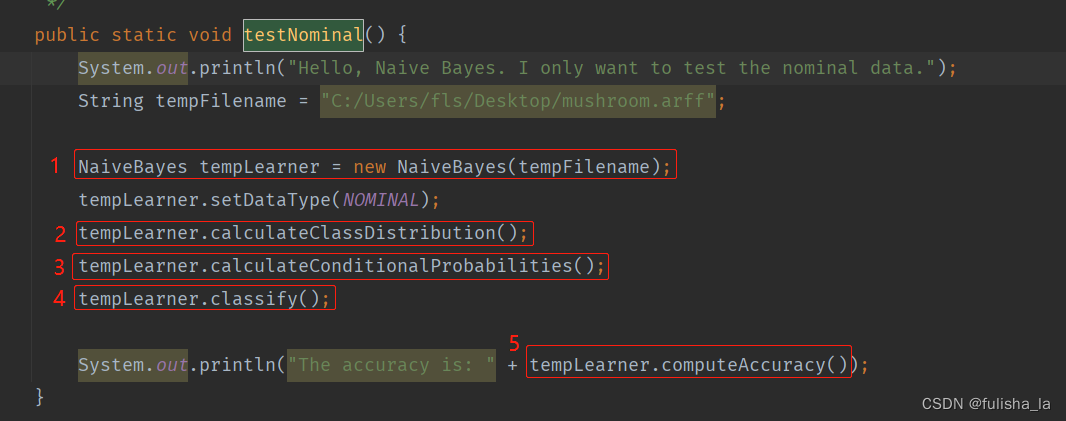
2.1.1 NaiveBayes 构造函数
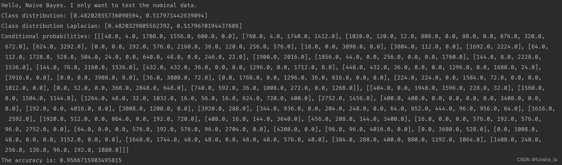
构造函数主要是读文本内容,初始化数据。可知mushroom.arff文件有8124条数据集,22个特征,2中类别选择。

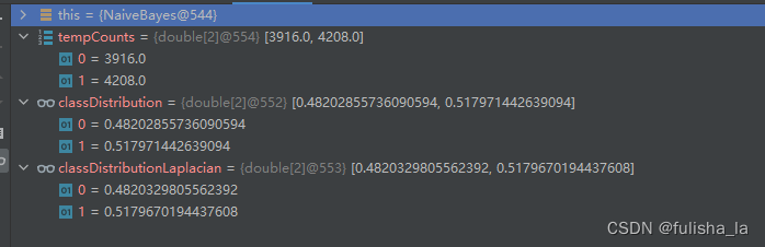
2.1.2 calculateClassDistribution()
计算类别分布概率。
- classDistribution 根据数据集计算不同类别的概率(就像上面我出去玩的概率是0.482028,不出去玩的概率是0.51797类似)
- classDistributionLaplacian 是对classDistribution 进行拉普拉斯平滑后的类别分布
2.1.3 calculateConditionalProbabilities()方法
- 进行空间分配(conditionalCounts和conditionalProbabilitiesLaplacian变量在初始分配都一样)
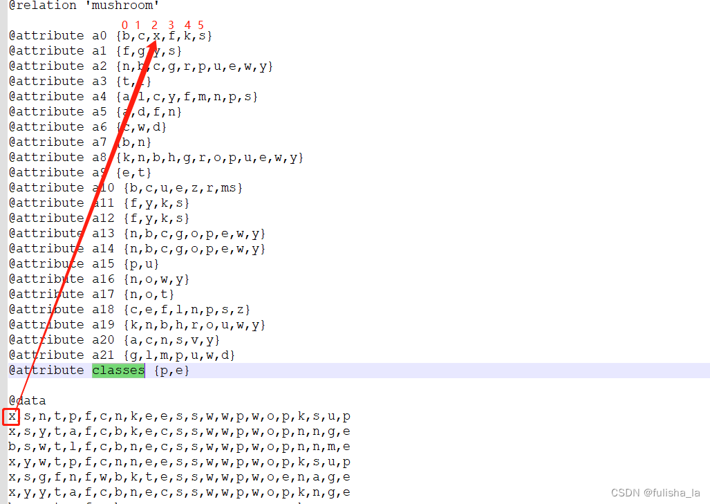
一共有22个特征,其实对比文件和代码的赋值就一目了然了
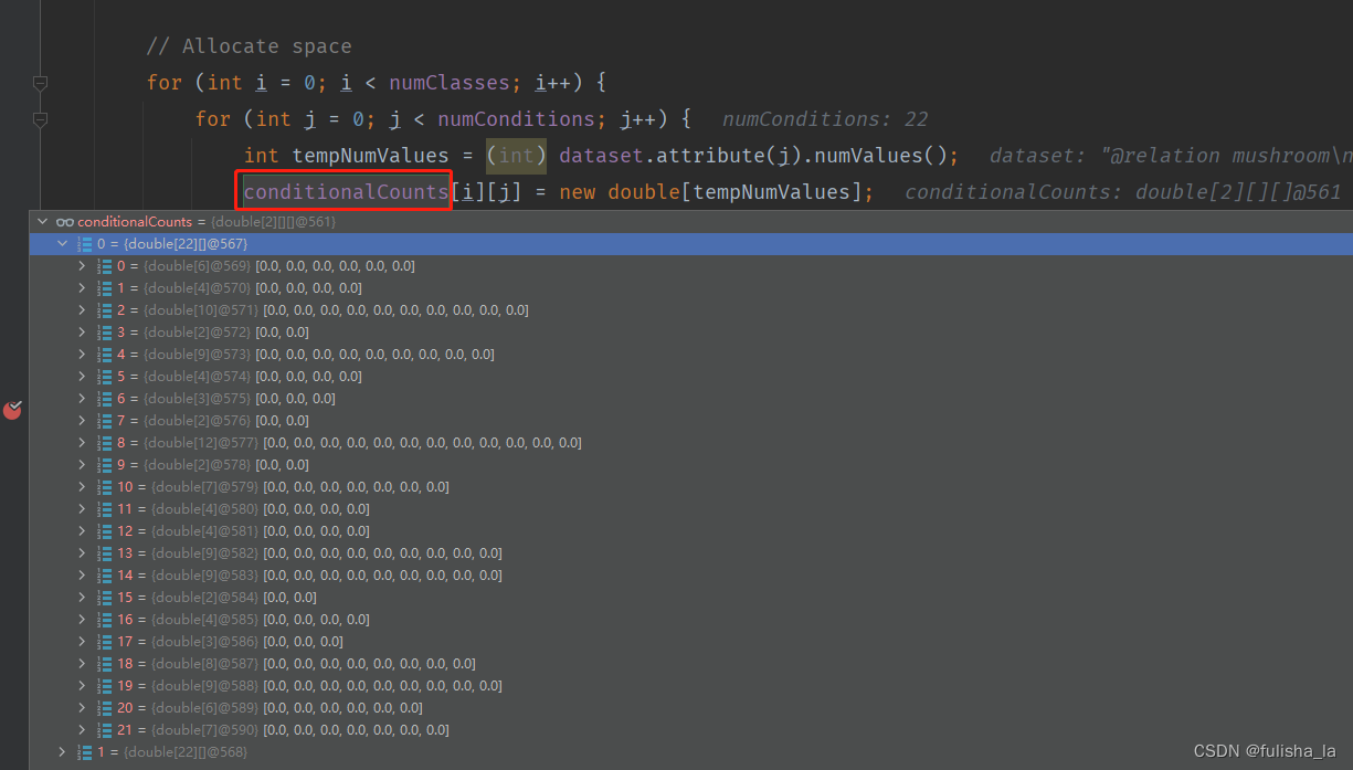
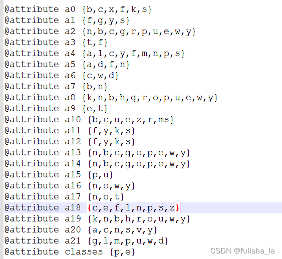
- conditionalCounts赋值
我也是看了好一会儿才明白这个取值。就如我们以conditionalCounts[0][0][tempValue]来理解,这个的含义就是我们第一行的数据中的第一个特征值即值为x,x所在的索引为2,conditionalCounts[0][0][2] 就累加一个1。同理conditionalCounts[0][1][tempValue]就是看他第2个特征值所在的索引位置是多少,以此类推

结合原数据来看
- 统计8124个数据样本出现在每个特征的次数(目的是为了方便计算后面的条件概率)

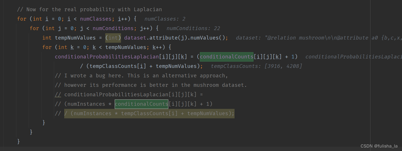
- 计算条件概率(conditionalProbabilitiesLaplacian赋值)(用Laplacian平滑)
结合上面Laplacian平滑基础知识即可,计算每个特征值出现的条件概率

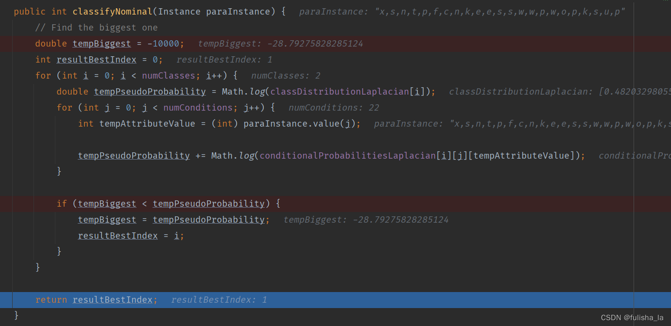
2.1.4 classify()方法
预测类别。在之前的代码中,已经把所有数据都准备好了,现在是结合这个公式去预测类别
就如我们预测文本中这个数据行:x,s,n,t,p,f,c,n,k,e,e,s,s,w,w,p,w,o,p,k,s,u,p,我们根据上面这个公式预测出的结果是他类别为e即1(实际上他类别为p即0)
2.1.5 computeAccuracy() 计算精确性
    /**
     * Compute accuracy.
     * @return
     */
    public double computeAccuracy() {
        double tempCorrect = 0;
        for (int i = 0; i < numInstances; i++) {
            if (predicts[i] == (int) dataset.instance(i).classValue()) {
                tempCorrect++;
            }
        }

        double resultAccuracy = tempCorrect / numInstances;
        return resultAccuracy;
    }
代码结果:全部代码可以看文章链接。
Day59 数值型数据的 NB 算法
1.基础理论知识
1.1 数值型和符号型NB 对比
- 符号型的NB算法适用于处理离散型的符号特征,概率分布是离散的,并且通过计算特征在给定类别下的频率来估计条件概率
- 数值型的NB算法适用于处理连续性的数值特征,假设特征的概率分布符合某个已知的概率分布(通常是高斯分布,高斯分布是连续型随机变量最常见的概率分布),通过计算给定类别下特征的概率密度函数,进而计算条件概率(会涉及计算均值和标准差)
例如:针对符号性,我们假设天气的状况是:晴朗,阴天,下雨等;而对数值型我们假设天气是根据温度具体是多少度。- 我们计算符号型的NB算法:我们可以计算每个天气状况下出去玩或不出去玩的概率,对于给定的天气状况,我们可以计算该状况在每个类别下的条件概率。
- 我们计算数值型NB算法:我们可以计算出去玩和不出去玩下温度的均值和方差,对于给定的温度,我们可以使用高斯分布的概率密度函数计算该温度在每个类别下的条件概率
1.2高斯分布(正态分布)
- 概率密度函数
随机变量X服从一个位置参数为 μ \mu μ、尺度参数为 σ \sigma σ 的概率分布,且其概率密度函数
p ( x ) = 1 2 π σ e x p ( − ( x − u ) 2 2 σ 2 ) p(x)=\frac{1}{\sqrt{2\pi\sigma}}exp({-\frac{(x-u)^{2}}{2\sigma ^{2}}}) p(x)=2πσ1exp(−2σ2(x−u)2)
均值 μ \mu μ的计算方法:对于已有的数据集,均值表示数据的平均值μ = (x₁ + x₂ + … + xₙ) / n
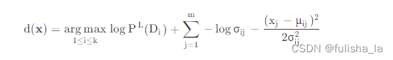
标准差 σ \sigma σ,数据集的离散程度,是观测值与均值之间的平均差异. σ = Σ ( x − u ) 2 n \sigma =\sqrt{\frac{\Sigma(x-u) ^{2}}{n}} σ=nΣ(x−u)2 - 预测方案修改
我们预测某个特征值下,Di发生的概率,公式如下
p ( D i ∣ x ) = p ( x D i ) p ( x ) = p ( D i ) p ( x ∣ D i ) p ( x ) = p ( D i ) ∏ j = 1 m p ( x j ∣ D i ) p ( x ) p(D_{i}|x)= \frac{p(xD_{i})}{p(x)}=\frac{p(D_{i})p(x|D_{i})}{p(x)}=\frac{p(D_{i})\prod_{j=1}^{m}p(x_{j}|D_{i})}{p(x)} p(Di∣x)=p(x)p(xDi)=p(x)p(Di)p(x∣Di)=p(x)p(Di)∏j=1mp(xj∣Di) 在符号型NB算法下,我们的预测方案中 p ( x j ∣ D i ) p(x_{j}|D_{i}) p(xj∣Di)我们可以求出来,其中现在对连续性数值, p ( x j ∣ D i ) p(x_{j}|D_{i}) p(xj∣Di)的计算很显然计算不出来,所以引入高斯分布替换调 p ( x j ∣ D i ) p(x_{j}|D_{i}) p(xj∣Di),而用相应的概率密度函数。所以对符号型NB算法中的预测方案d(x)进行修改,并对等式两边同样是取对数,则预测方案如下
2.符号型数据的预测算法跟踪
同样我也debug看一下
2.1 testNumerical()方法
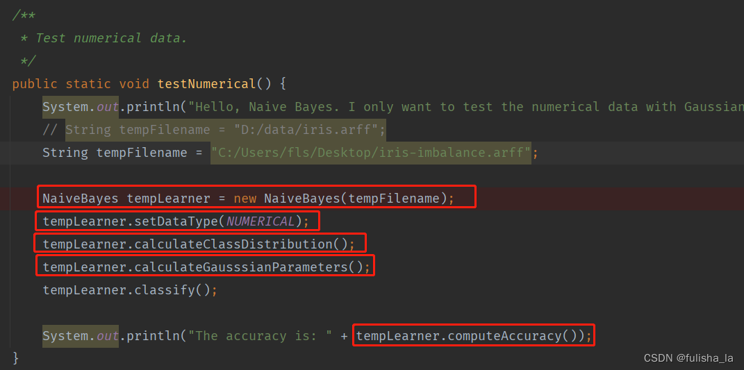
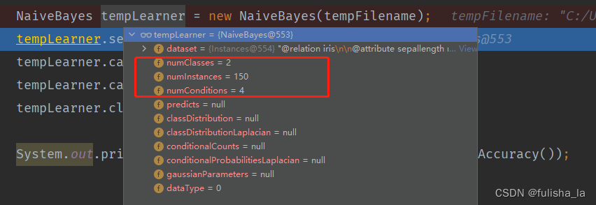
2.1.1 构造方法NaiveBayes
与符号型代码无差 目前给出的样本是有150个数据集,4个特征,2个类别。
2.1.2 calculateClassDistribution()
与符号型代码无差
2.1.3 calculateGausssianParameters()方法
计算条件概率(采用高斯分布)
- gaussianParameters变量
存储每个类别下,不同特征值的高斯参数,包含均值,标准差。如下是这个方法执行完存储的值。
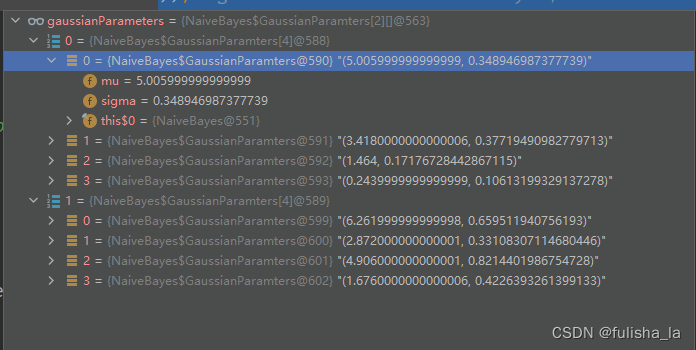
- 方法中的循环则是对gaussianParameters中赋值
计算不同类别下,不同特征值的均值和标准差。
 public void calculateGausssianParameters() {
        gaussianParameters = new GaussianParamters[numClasses][numConditions];

        double[] tempValuesArray = new double[numInstances];
        int tempNumValues = 0;
        double tempSum = 0;

        for (int i = 0; i < numClasses; i++) {
            for (int j = 0; j < numConditions; j++) {
                tempSum = 0;

                // Obtain values for this class.
                tempNumValues = 0;
                for (int k = 0; k < numInstances; k++) {
                    if ((int) dataset.instance(k).classValue() != i) {
                        continue;
                    }

                    tempValuesArray[tempNumValues] = dataset.instance(k).value(j);
                    tempSum += tempValuesArray[tempNumValues];
                    tempNumValues++;
                }

                // Obtain parameters.
                double tempMu = tempSum / tempNumValues;

                double tempSigma = 0;
                for (int k = 0; k < tempNumValues; k++) {
                    tempSigma += (tempValuesArray[k] - tempMu) * (tempValuesArray[k] - tempMu);
                }
                tempSigma /= tempNumValues;
                tempSigma = Math.sqrt(tempSigma);

                gaussianParameters[i][j] = new GaussianParamters(tempMu, tempSigma);
            }
        }

        System.out.println(Arrays.deepToString(gaussianParameters));
    }
2.1.4 classify()方法
预测类别。在之前的代码中,已经把所有数据都准备好了,现在是结合这个公式去预测类别
代码运行结果。
我想说这个的预测的精准率有点高呀~直接100%了
如果我将读入文本换为之前的iris.arff,结果如下
全部代码:
package machinelearing;

import weka.core.Instance;
import weka.core.Instances;

import java.io.FileReader;
import java.util.Arrays;
import java.util.Random;

/**
 * @author: fulisha
 * @date: 2023/6/2 9:22
 * @description:
 */
public class NaiveBayes {
    /**
     * An inner class to store parameters.
     */
    private class GaussianParamters {
        double mu;
        double sigma;

        public GaussianParamters(double paraMu, double paraSigma) {
            mu = paraMu;
            sigma = paraSigma;
        }

        @Override
        public String toString() {
            return "(" + mu + ", " + sigma + ")";
        }
    }

    /**
     * The data.
     */
    Instances dataset;

    /**
     * The number of classes. For binary classification it is 2.
     */
    int numClasses;

    /**
     * The number of instances.
     */
    int numInstances;

    /**
     * The number of conditional attributes.
     */
    int numConditions;

    /**
     * The prediction, including queried and predicted labels.
     */
    int[] predicts;

    /**
     * Class distribution.
     */
    double[] classDistribution;

    /**
     * Class distribution with Laplacian smooth.
     */
    double[] classDistributionLaplacian;

    /**
     * To calculate the conditional probabilities for all classes over all
     * attributes on all values.
     */
    double[][][] conditionalCounts;

    /**
     * The conditional probabilities with Laplacian smooth.
     */
    double[][][] conditionalProbabilitiesLaplacian;

    /**
     * The Guassian parameters.
     */
    GaussianParamters[][] gaussianParameters;

    /**
     * Data type.
     */
    int dataType;

    /**
     * Nominal.
     */
    public static final int NOMINAL = 0;

    /**
     * Numerical.
     */
    public static final int NUMERICAL = 1;


    /**
     * The constructor
     * @param paraFileName The given file.
     */
    public NaiveBayes(String paraFileName) {
        dataset = null;
        try {
            FileReader reader = new FileReader(paraFileName);
            dataset = new Instances(reader);
            reader.close();
        }catch (Exception e) {
            System.out.println("Cannot read the file: " + paraFileName + "\r\n" + e);
            System.exit(0);
        }

        dataset.setClassIndex(dataset.numAttributes() - 1);
        numConditions = dataset.numAttributes() - 1;
        numInstances = dataset.numInstances();
        numClasses = dataset.attribute(numConditions).numValues();
    }

    /**
     * The constructor
     * @param paraInstances  The given file.
     */
    public NaiveBayes(Instances paraInstances) {
        dataset = paraInstances;

        dataset.setClassIndex(dataset.numAttributes() - 1);
        numConditions = dataset.numAttributes() - 1;
        numInstances = dataset.numInstances();
        numClasses = dataset.attribute(numConditions).numValues();
    }

    /**
     * Set the data type.
     * @param paraDataType
     */
    public void setDataType(int paraDataType) {
        dataType = paraDataType;
    }

    /**
     * Calculate the class distribution with Laplacian smooth.
     */
    public void calculateClassDistribution() {
        classDistribution = new double[numClasses];
        classDistributionLaplacian = new double[numClasses];

        double[] tempCounts = new double[numClasses];
        for (int i = 0; i < numInstances; i++) {
            int tempClassValue = (int) dataset.instance(i).classValue();
            tempCounts[tempClassValue]++;
        }

        for (int i = 0; i < numClasses; i++) {
            classDistribution[i] = tempCounts[i] / numInstances;
            classDistributionLaplacian[i] = (tempCounts[i] + 1) / (numInstances + numClasses);
        }

        System.out.println("Class distribution: " + Arrays.toString(classDistribution));
        System.out.println("Class distribution Laplacian: " + Arrays.toString(classDistributionLaplacian));
    }


    /**
     *  Calculate the conditional probabilities with Laplacian smooth. ONLY scan the dataset once.
     *  There was a simpler one, I have removed it because the time complexity is higher.
     */
    public void calculateConditionalProbabilities() {
        conditionalCounts = new double[numClasses][numConditions][];
        conditionalProbabilitiesLaplacian = new double[numClasses][numConditions][];

        // Allocate space
        for (int i = 0; i < numClasses; i++) {
            for (int j = 0; j < numConditions; j++) {
                int tempNumValues = (int) dataset.attribute(j).numValues();
                conditionalCounts[i][j] = new double[tempNumValues];
                conditionalProbabilitiesLaplacian[i][j] = new double[tempNumValues];
            }
        }

        // Count the numbers
        int[] tempClassCounts = new int[numClasses];
        for (int i = 0; i < numInstances; i++) {
            int tempClass = (int) dataset.instance(i).classValue();
            tempClassCounts[tempClass]++;
            for (int j = 0; j < numConditions; j++) {
                int tempValue = (int) dataset.instance(i).value(j);
                conditionalCounts[tempClass][j][tempValue]++;
            }
        }

        // Now for the real probability with Laplacian
        for (int i = 0; i < numClasses; i++) {
            for (int j = 0; j < numConditions; j++) {
                int tempNumValues = (int) dataset.attribute(j).numValues();
                for (int k = 0; k < tempNumValues; k++) {
                    conditionalProbabilitiesLaplacian[i][j][k] = (conditionalCounts[i][j][k] + 1)
                            / (tempClassCounts[i] + tempNumValues);
                    // I wrote a bug here. This is an alternative approach,
                    // however its performance is better in the mushroom dataset.
                    // conditionalProbabilitiesLaplacian[i][j][k] =
                    // (numInstances * conditionalCounts[i][j][k] + 1)
                    // / (numInstances * tempClassCounts[i] + tempNumValues);
                }
            }
        }

        System.out.println("Conditional probabilities: " + Arrays.deepToString(conditionalCounts));
    }

    /**
     *  Calculate the conditional probabilities with Laplacian smooth.
     */
    public void calculateGausssianParameters() {
        gaussianParameters = new GaussianParamters[numClasses][numConditions];

        double[] tempValuesArray = new double[numInstances];
        int tempNumValues = 0;
        double tempSum = 0;

        for (int i = 0; i < numClasses; i++) {
            for (int j = 0; j < numConditions; j++) {
                tempSum = 0;

                // Obtain values for this class.
                tempNumValues = 0;
                for (int k = 0; k < numInstances; k++) {
                    if ((int) dataset.instance(k).classValue() != i) {
                        continue;
                    }

                    tempValuesArray[tempNumValues] = dataset.instance(k).value(j);
                    tempSum += tempValuesArray[tempNumValues];
                    tempNumValues++;
                }

                // Obtain parameters.
                double tempMu = tempSum / tempNumValues;

                double tempSigma = 0;
                for (int k = 0; k < tempNumValues; k++) {
                    tempSigma += (tempValuesArray[k] - tempMu) * (tempValuesArray[k] - tempMu);
                }
                tempSigma /= tempNumValues;
                tempSigma = Math.sqrt(tempSigma);

                gaussianParameters[i][j] = new GaussianParamters(tempMu, tempSigma);
            }
        }

        System.out.println(Arrays.deepToString(gaussianParameters));
    }

    /**
     *  Classify all instances, the results are stored in predicts[].
     */
    public void classify() {
        predicts = new int[numInstances];
        for (int i = 0; i < numInstances; i++) {
            predicts[i] = classify(dataset.instance(i));
        }
    }

    public int classify(Instance paraInstance) {
        if (dataType == NOMINAL) {
            return classifyNominal(paraInstance);
        } else if (dataType == NUMERICAL) {
            return classifyNumerical(paraInstance);
        } // Of if

        return -1;
    }

    /**
     * Classify an instances with nominal data.
     * @param paraInstance
     * @return
     */
    public int classifyNominal(Instance paraInstance) {
        // Find the biggest one
        double tempBiggest = -10000;
        int resultBestIndex = 0;
        for (int i = 0; i < numClasses; i++) {
            double tempPseudoProbability = Math.log(classDistributionLaplacian[i]);
            for (int j = 0; j < numConditions; j++) {
                int tempAttributeValue = (int) paraInstance.value(j);

                tempPseudoProbability += Math.log(conditionalProbabilitiesLaplacian[i][j][tempAttributeValue]);
            }

            if (tempBiggest < tempPseudoProbability) {
                tempBiggest = tempPseudoProbability;
                resultBestIndex = i;
            }
        }

        return resultBestIndex;
    }

    /**
     * Classify an instances with numerical data.
     * @param paraInstance
     * @return
     */
    public int classifyNumerical(Instance paraInstance) {
        // Find the biggest one
        double tempBiggest = -10000;
        int resultBestIndex = 0;

        for (int i = 0; i < numClasses; i++) {
            double tempPseudoProbability = Math.log(classDistributionLaplacian[i]);
            for (int j = 0; j < numConditions; j++) {
                double tempAttributeValue = paraInstance.value(j);
                double tempSigma = gaussianParameters[i][j].sigma;
                double tempMu = gaussianParameters[i][j].mu;

                tempPseudoProbability += -Math.log(tempSigma)
                        - (tempAttributeValue - tempMu) * (tempAttributeValue - tempMu) / (2 * tempSigma * tempSigma);
            }

            if (tempBiggest < tempPseudoProbability) {
                tempBiggest = tempPseudoProbability;
                resultBestIndex = i;
            }
        }

        return resultBestIndex;
    }

    /**
     * Compute accuracy.
     * @return
     */
    public double computeAccuracy() {
        double tempCorrect = 0;
        for (int i = 0; i < numInstances; i++) {
            if (predicts[i] == (int) dataset.instance(i).classValue()) {
                tempCorrect++;
            }
        }

        double resultAccuracy = tempCorrect / numInstances;
        return resultAccuracy;
    }

    /**
     *  Test nominal data.
     */
    public static void testNominal() {
        System.out.println("Hello, Naive Bayes. I only want to test the nominal data.");
        String tempFilename = "C:/Users/fls/Desktop/mushroom.arff";

        NaiveBayes tempLearner = new NaiveBayes(tempFilename);
        tempLearner.setDataType(NOMINAL);
        tempLearner.calculateClassDistribution();
        tempLearner.calculateConditionalProbabilities();
        tempLearner.classify();

        System.out.println("The accuracy is: " + tempLearner.computeAccuracy());
    }

    /**
     * Test numerical data.
     */
    public static void testNumerical() {
        System.out.println("Hello, Naive Bayes. I only want to test the numerical data with Gaussian assumption.");
        // String tempFilename = "D:/data/iris.arff";
        String tempFilename = "C:/Users/fls/Desktop/iris.arff";

        NaiveBayes tempLearner = new NaiveBayes(tempFilename);
        tempLearner.setDataType(NUMERICAL);
        tempLearner.calculateClassDistribution();
        tempLearner.calculateGausssianParameters();
        tempLearner.classify();

        System.out.println("The accuracy is: " + tempLearner.computeAccuracy());
    }

    /**
     * Test this class.
     * @param args
     */
    public static void main(String[] args) {
        testNominal();
        testNumerical();
        // testNominal(0.8);
    }

    /**
     * Get a random indices for data randomization.
     * @param paraLength  The length of the sequence.
     * @return An array of indices, e.g., {4, 3, 1, 5, 0, 2} with length 6.
     */
    public static int[] getRandomIndices(int paraLength) {
        Random random = new Random();
        int[] resultIndices = new int[paraLength];

        // Step 1. Initialize.
        for (int i = 0; i < paraLength; i++) {
            resultIndices[i] = i;
        } // Of for i

        // Step 2. Randomly swap.
        int tempFirst, tempSecond, tempValue;
        for (int i = 0; i < paraLength; i++) {
            // Generate two random indices.
            tempFirst = random.nextInt(paraLength);
            tempSecond = random.nextInt(paraLength);

            // Swap.
            tempValue = resultIndices[tempFirst];
            resultIndices[tempFirst] = resultIndices[tempSecond];
            resultIndices[tempSecond] = tempValue;
        } // Of for i

        return resultIndices;
    }

    /**
     * Split the data into training and testing parts.
     * @param paraDataset
     * @param paraTrainingFraction The fraction of the training set.
     * @return
     */
    public static Instances[] splitTrainingTesting(Instances paraDataset, double paraTrainingFraction) {
        int tempSize = paraDataset.numInstances();
        int[] tempIndices = getRandomIndices(tempSize);
        int tempTrainingSize = (int) (tempSize * paraTrainingFraction);

        // Empty datasets.
        Instances tempTrainingSet = new Instances(paraDataset);
        tempTrainingSet.delete();
        Instances tempTestingSet = new Instances(tempTrainingSet);

        for (int i = 0; i < tempTrainingSize; i++) {
            tempTrainingSet.add(paraDataset.instance(tempIndices[i]));
        } // Of for i

        for (int i = 0; i < tempSize - tempTrainingSize; i++) {
            tempTestingSet.add(paraDataset.instance(tempIndices[tempTrainingSize + i]));
        } // Of for i

        tempTrainingSet.setClassIndex(tempTrainingSet.numAttributes() - 1);
        tempTestingSet.setClassIndex(tempTestingSet.numAttributes() - 1);
        Instances[] resultInstanesArray = new Instances[2];
        resultInstanesArray[0] = tempTrainingSet;
        resultInstanesArray[1] = tempTestingSet;

        return resultInstanesArray;
    }


    /**
     * Classify all instances, the results are stored in predicts[].
     * @param paraTestingSet
     * @return
     */
    public double classify(Instances paraTestingSet) {
        double tempCorrect = 0;
        int[] tempPredicts = new int[paraTestingSet.numInstances()];
        for (int i = 0; i < tempPredicts.length; i++) {
            tempPredicts[i] = classify(paraTestingSet.instance(i));
            if (tempPredicts[i] == (int) paraTestingSet.instance(i).classValue()) {
                tempCorrect++;
            } // Of if
        } // Of for i

        System.out.println("" + tempCorrect + " correct over " + tempPredicts.length + " instances.");
        double resultAccuracy = tempCorrect / tempPredicts.length;
        return resultAccuracy;
    }

    /**
     * Test nominal data.
     * @param paraTrainingFraction
     */
    public static void testNominal(double paraTrainingFraction) {
        System.out.println("Hello, Naive Bayes. I only want to test the nominal data.");
        String tempFilename = "D:/data/mushroom.arff";
        // String tempFilename = "D:/data/voting.arff";

        Instances tempDataset = null;
        try {
            FileReader fileReader = new FileReader(tempFilename);
            tempDataset = new Instances(fileReader);
            fileReader.close();
        } catch (Exception ee) {
            System.out.println("Cannot read the file: " + tempFilename + "\r\n" + ee);
            System.exit(0);
        } // Of try

        Instances[] tempDatasets = splitTrainingTesting(tempDataset, paraTrainingFraction);
        NaiveBayes tempLearner = new NaiveBayes(tempDatasets[0]);
        tempLearner.setDataType(NOMINAL);
        tempLearner.calculateClassDistribution();
        tempLearner.calculateConditionalProbabilities();

        double tempAccuracy = tempLearner.classify(tempDatasets[1]);

        System.out.println("The accuracy is: " + tempAccuracy);
    }
}