博主前期相关的博客见下：
cs109-energy+哈佛大学能源探索项目 Part-1（项目背景）
这次主要讲数据的整理。

Data Wrangling

数据整理

在哈佛的一些大型建筑中，有三种类型的能源消耗，电力，冷冻水和蒸汽。 冷冻水是用来冷却的，蒸汽是用来加热的。下图显示了哈佛工厂提供冷冻水和蒸汽的建筑。
在这里插入图片描述

Fig. Harvard chilled water and steam supply. (Left: chilled water, highlighted in blue. Right: Steam, highlighted in yellow）
图：哈佛的冷冻水和蒸汽供应。(左图：冷冻水，用蓝色突出显示。右边：蒸汽，以黄色标示）。

我们选取了一栋建筑，得到了2011年07月01日至2014年10月31日的能耗数据。由于仪表故障，有几个月的数据丢失了。数据分辨率为每小时。在原始数据中，每小时的数据是仪表读数。为了得到每小时的消耗量，我们需要抵消数据，做减法。我们有从2012年1月到2014年10月每小时的天气和能源数据(2.75年)。这些天气数据来自剑桥的气象站。

在本节中，我们将完成以下任务。
1、从Harvard Energy Witness website上手动下载原始数据，获取每小时的电力、冷冻水和蒸汽。
2、清洁的天气数据，增加更多的功能，包括冷却度，加热度和湿度比。
3、根据假期、学年和周末估计每日入住率。
4、创建与小时相关的特征，即cos(hourOfDay 2 pi / 24)。
5、将电、冷冻水和蒸汽数据框与天气、时间和占用特性相结合。

数据下载

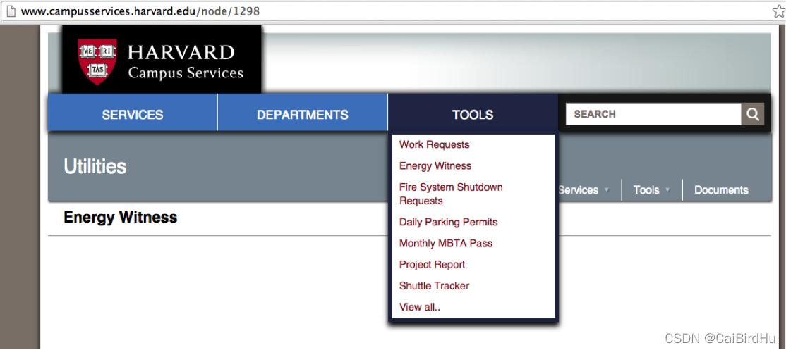
原始数据从(Harvard Energy Witness Website)下载
Energy Witness

PASS：该网站目前无法获取数据
后面部分主要学习其分析数据的技巧

在这里插入图片描述

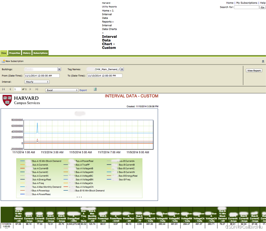
然后我们使用Pandas把它们放在 one dataframe。

file = 'Data/Org/0701-0930-2011.xls' 
df = pd.read_excel(file, header = 0, skiprows = np.arange(0,6))

files = ['Data/Org/1101-1130-2011.xls', 'Data/Org/1201-2011-0131-2012.xls',
         'Data/Org/0201-0331-2012.xls','Data/Org/0401-0531-2012.xls','Data/Org/0601-0630-2012.xls',
         'Data/Org/0701-0831-2012.xls','Data/Org/0901-1031-2012.xls','Data/Org/1101-1231-2012.xls',
         'Data/Org/0101-0228-2013.xls',
         'Data/Org/0301-0430-2013.xls','Data/Org/0501-0630-2013.xls','Data/Org/0701-0831-2013.xls',
         'Data/Org/0901-1031-2013.xls','Data/Org/1101-1231-2013.xls','Data/Org/0101-0228-2014.xls',
         'Data/Org/0301-0430-2014.xls', 'Data/Org/0501-0630-2014.xls', 'Data/Org/0701-0831-2014.xls',
         'Data/Org/0901-1031-2014.xls']

for file in files:
    data = pd.read_excel(file, header = 0, skiprows = np.arange(0,6))
    df = df.append(data)

df.head()

这段代码的作用是将多个 Excel 文件中的数据读取到一个 DataFrame 中。首先，使用 Pandas 的 read_excel 函数读取 Data/Org/0701-0930-2011.xls 文件中的数据，并指定参数 header = 0 和 skiprows = np.arange(0,6)，其中 header = 0 表示将第一行作为表头，skiprows = np.arange(0,6) 表示跳过前六行（通常是一些无用的信息或标题）。将读取的数据存储在 df 变量中。

接下来，定义了一个文件名列表 files，包含了要读取的所有 Excel 文件名。然后使用 for 循环逐一读取这些文件中的数据，将每个文件的数据存储在变量 data 中，再通过 append 方法将 data 中的数据添加到 df 变量中，最终得到一个包含所有文件数据的 DataFrame。

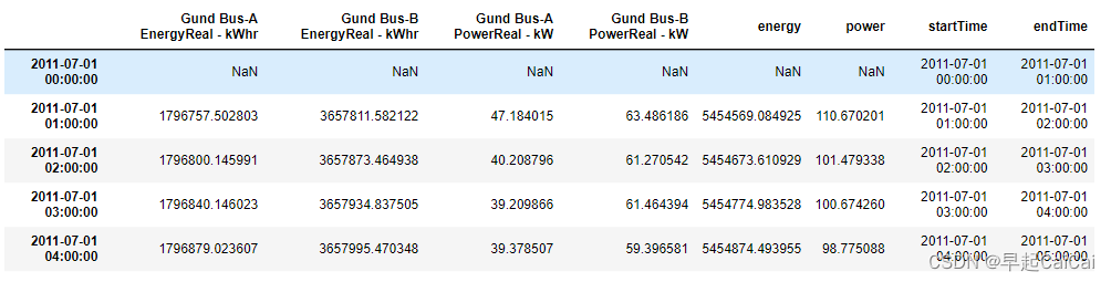
以上是原始的小时数据。
如你所见，非常混乱。移除无意义列的第一件事。

df.rename(columns={'Unnamed: 0':'Datetime'}, inplace=True)
nonBlankColumns = ['Unnamed' not in s for s in df.columns]
columns = df.columns[nonBlankColumns]
df = df[columns]
df = df.set_index(['Datetime'])
df.index.name = None
df.head()

这段代码做了以下事情：

将 Unnamed: 0'这一列的列名改为 Datetime。
创建一个布尔列表 nonBlankColumns，其中包含所有列名中不包含 Unnamed 的列。
选择所有布尔列表中为 True 的列名，并将其存储在一个新的 columns 变量中。
删除所有非空列（即 nonBlankColumns 中为 False 的列）。
将 Datetime列设置为索引。
将索引名称更改为 None。
返回 DataFrame 的前五行。

然后我们打印出所有的列名。只有少数几列是有用的，以获取每小时的电，冷冻水和蒸汽。

for item in df.columns:
    print item

Electricity

以电力为例，有两个计量器，“Gund Bus A"和"Gund Bus B”。"EnergyReal-kWhr"记录了累积用电量。我们不确定"PoweReal"确切代表什么。为了以防万一，我们也将其放入电力数据框中。

electricity=df[['Gund Bus-A EnergyReal - kWhr','Gund Bus-B EnergyReal - kWhr',
                'Gund Bus-A PowerReal - kW','Gund Bus-B PowerReal - kW',]]
electricity.head()

在这里插入图片描述

Validate our data processing method by checking monthly energy consumption

通过月度能耗检查，验证数据处理方法

为了检验我们对数据的理解是否正确，我们想从小时数据计算出每月的用电量，然后将结果与facalities提供的每月数据进行比较，facalities也可以在Energy Witness上找到。

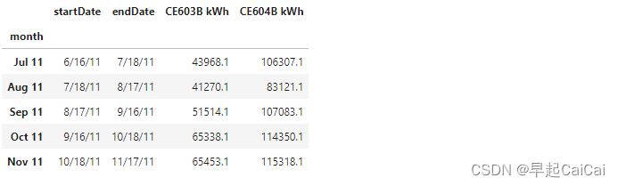
这是设施提供的月度数据，“Bus A和B”在这个月度表格中被称为“CE603B kWh”和“CE604B kWh”。它们只是两个电表。请注意，电表读数周期不是按照日历月计算的。

file = 'Data/monthly electricity.csv' 
monthlyElectricityFromFacility = pd.read_csv(file, header=0)
monthlyElectricityFromFacility = monthlyElectricityFromFacility.set_index(['month'])
monthlyElectricityFromFacility.head()

这段代码用于读取一个名为 “monthly electricity.csv” 的文件，并将其转换为一个名为 monthlyElectricityFromFacility 的 Pandas 数据帧对象。在读取文件时，header=0参数表示将第一行视为数据帧的列标题。然后，将 “month” 列作为数据帧的索引列，使用 set_index() 方法来完成。最后，用 head() 方法来显示数据帧的前五行。

在这里插入图片描述

我们使用两个电表的“EnergyReal - kWhr”列。我们找到了电表读数周期的开始和结束日期的编号，然后用结束日期的编号减去开始日期的编号，就得到了每月的用电量。

monthlyElectricityFromFacility['startDate'] = pd.to_datetime(monthlyElectricityFromFacility['startDate'], format="%m/%d/%y")
values = monthlyElectricityFromFacility.index.values

keys = np.array(monthlyElectricityFromFacility['startDate'])

dates = {}
for key, value in zip(keys, values):
    dates[key] = value

sortedDates =  np.sort(dates.keys())
sortedDates = sortedDates[sortedDates > np.datetime64('2011-11-01')]

months = []
monthlyElectricityOrg = np.zeros((len(sortedDates) - 1, 2))
for i in range(len(sortedDates) - 1):
    begin = sortedDates[i]
    end = sortedDates[i+1]
    months.append(dates[sortedDates[i]])
    monthlyElectricityOrg[i, 0] = (np.round(electricity.loc[end,'Gund Bus-A EnergyReal - kWhr'] 
                           -  electricity.loc[begin,'Gund Bus-A EnergyReal - kWhr'], 1))
    monthlyElectricityOrg[i, 1] = (np.round(electricity.loc[end,'Gund Bus-B EnergyReal - kWhr'] 
                           -  electricity.loc[begin,'Gund Bus-B EnergyReal - kWhr'], 1))

monthlyElectricity = pd.DataFrame(data = monthlyElectricityOrg, index = months, columns = ['CE603B kWh', 'CE604B kWh'])


plt.figure()
fig, ax = plt.subplots()
fig = monthlyElectricity.plot(marker = 'o', figsize=(15,6), rot = 40, fontsize = 13, ax = ax, linestyle='')
fig.set_axis_bgcolor('w')
plt.xlabel('Billing month', fontsize = 15)
plt.ylabel('kWh', fontsize = 15)
plt.tick_params(which=u'major', reset=False, axis = 'y', labelsize = 13)
plt.xticks(np.arange(0,len(months)),months)
plt.title('Original monthly consumption from hourly data',fontsize = 17)

text = 'Meter malfunction'
ax.annotate(text, xy = (9, 4500000), 
            xytext = (5, 2), fontsize = 15,
            textcoords = 'offset points', ha = 'center', va = 'top')

ax.annotate(text, xy = (8, -4500000), 
            xytext = (5, 2), fontsize = 15, 
            textcoords = 'offset points', ha = 'center', va = 'bottom')

ax.annotate(text, xy = (14, -2500000), 
            xytext = (5, 2), fontsize = 15, 
            textcoords = 'offset points', ha = 'center', va = 'bottom')

ax.annotate(text, xy = (15, 2500000), 
            xytext = (5, 2), fontsize = 15, 
            textcoords = 'offset points', ha = 'center', va = 'top')

plt.show()

以下是代码的解释：

monthlyElectricityFromFacility['startDate'] = pd.to_datetime(monthlyElectricityFromFacility['startDate'], format="%m/%d/%y")

将monthlyElectricityFromFacility数据框中的"startDate"列转换为datetime类型，并指定日期格式为"%m/%d/%y"。

values = monthlyElectricityFromFacility.index.values
keys = np.array(monthlyElectricityFromFacility['startDate'])

将monthlyElectricityFromFacility数据框的索引值保存到values中，并将"startDate"列的值保存到keys中。

dates = {}
for key, value in zip(keys, values):
    dates[key] = value

创建一个名为dates的字典，将"startDate"列的值作为键，索引值作为值存储到dates字典中。

sortedDates =  np.sort(dates.keys())
sortedDates = sortedDates[sortedDates > np.datetime64('2011-11-01')]

将dates字典的键按升序排序，并将排序后的结果保存到sortedDates中，然后从排序后的结果中筛选出大于2011年11月1日的日期。

months = []
monthlyElectricityOrg = np.zeros((len(sortedDates) - 1, 2))
for i in range(len(sortedDates) - 1):
    begin = sortedDates[i]
    end = sortedDates[i+1]
    months.append(dates[sortedDates[i]])
    monthlyElectricityOrg[i, 0] = (np.round(electricity.loc[end,'Gund Bus-A EnergyReal - kWhr'] 
                           -  electricity.loc[begin,'Gund Bus-A EnergyReal - kWhr'], 1))
    monthlyElectricityOrg[i, 1] = (np.round(electricity.loc[end,'Gund Bus-B EnergyReal - kWhr'] 
                           -  electricity.loc[begin,'Gund Bus-B EnergyReal - kWhr'], 1))

创建一个空列表months和一个形状为(len(sortedDates) - 1, 2)的全零数组monthlyElectricityOrg。然后遍历sortedDates中的每个日期，计算开始日期和结束日期之间的用电量，并将用电量保存到monthlyElectricityOrg数组中。同时，将每个月的名称保存到months列表中。

monthlyElectricity = pd.DataFrame(data = monthlyElectricityOrg, index = months, columns = ['CE603B kWh', 'CE604B kWh'])

将monthlyElectricityOrg数组转换为数据框，并将months列表作为索引，[‘CE603B kWh’, ‘CE604B kWh’]作为列名。

plt.figure()
fig, ax = plt.subplots()
fig = monthlyElectricity.plot(marker = 'o', figsize=(15,6), rot = 40, fontsize = 13, ax = ax, linestyle='')
fig.set_axis_bgcolor('w')
plt.xlabel('Billing month', fontsize = 15)
plt.ylabel('kWh', fontsize = 15)
plt.tick_params(which=u'major', reset=False, axis = 'y', labelsize = 13)
plt.xticks(np.arange(0,len(months)),months)
plt.title('Original monthly consumption from hourly data',fontsize = 17)

创建一个图形，并绘制monthlyElectricity数据框中的数据。设置x轴标签为"Billing month"，y轴标签为"kWh"，设置y轴标签字体大小为15。设置y轴刻度标签的字体大小为13，设置x轴刻度标签为months列表中的月份名称，并将x轴刻度标签旋转40度。设置图形标题为"Original monthly consumption from hourly data"，字体大小为17。

text = 'Meter malfunction'
ax.annotate(text, xy = (9, 4500000), 
            xytext = (5, 2), fontsize = 15,
            textcoords = 'offset points', ha = 'center', va = 'top')

ax.annotate(text, xy = (8, -4500000), 
            xytext = (5, 2), fontsize = 15, 
            textcoords = 'offset points', ha = 'center', va = 'bottom')

ax.annotate(text, xy = (14, -2500000), 
            xytext = (5, 2), fontsize = 15, 
            textcoords = 'offset points', ha = 'center', va = 'bottom')

ax.annotate(text, xy = (15, 2500000), 
            xytext = (5, 2), fontsize = 15, 
            textcoords = 'offset points', ha = 'center', va = 'top')

在图形上添加四个文本注释，分别位于坐标点(9, 4500000)、(8, -4500000)、(14, -2500000)和(15, 2500000)处，文本内容为"Meter malfunction"，字体大小为15，注释框的位置偏移量为(5, 2)。

在这里插入图片描述

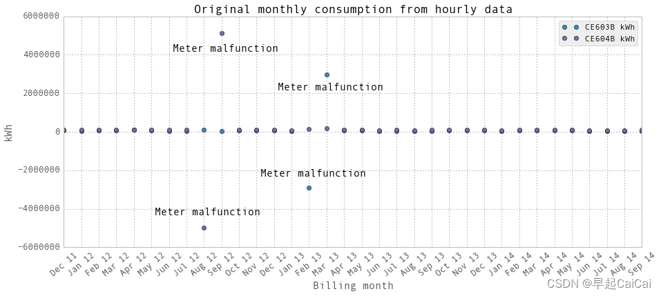
上面是使用我们的数据处理方法绘制的月度用电量图。显然，两个电表在几个月内发生了故障。图中有两组点，分别来自于两个电表，分别标注为"CE603B"和"CE604B"。建筑物的总用电量是这两个电表的电量之和。

图中的4个离群点为异常点

monthlyElectricity.loc['Aug 12','CE604B kWh'] = np.nan
monthlyElectricity.loc['Sep 12','CE604B kWh'] = np.nan
monthlyElectricity.loc['Feb 13','CE603B kWh'] = np.nan
monthlyElectricity.loc['Mar 13','CE603B kWh'] = np.nan


fig,ax = plt.subplots(1, 1,figsize=(15,8))
#ax.set_axis_bgcolor('w')
plt.bar(np.arange(0, len(monthlyElectricity))-0.5,monthlyElectricity['CE603B kWh'], label='Our data processing from hourly data')
plt.plot(monthlyElectricityFromFacility.loc[months,'CE603B kWh'],'or', label='Facility data')
plt.xticks(np.arange(0,len(months)),months)
plt.xlabel('Month',fontsize=15)
plt.ylabel('kWh',fontsize=15)
plt.xlim([0, len(monthlyElectricity)])
plt.legend()
ax.set_xticklabels(months, rotation=40, fontsize=13)
plt.tick_params(which=u'major', reset=False, axis = 'y', labelsize = 15)
plt.title('Comparison between our data processing and facilities, Meter CE603B',fontsize=20)

text = 'Meter malfunction \n estimated by facility'
ax.annotate(text, xy = (14, monthlyElectricityFromFacility.loc['Feb 13','CE603B kWh']), 
            xytext = (5, 50), fontsize = 15, 
            arrowprops=dict(facecolor='black', shrink=0.15),
            textcoords = 'offset points', ha = 'center', va = 'bottom')

ax.annotate(text, xy = (15, monthlyElectricityFromFacility.loc['Mar 13','CE603B kWh']), 
            xytext = (5, 50), fontsize = 15, 
            arrowprops=dict(facecolor='black', shrink=0.15),
            textcoords = 'offset points', ha = 'center', va = 'bottom')
plt.show()

fig,ax = plt.subplots(1, 1,figsize=(15,8))
#ax.set_axis_bgcolor('w')
plt.bar(np.arange(0, len(monthlyElectricity))-0.5, monthlyElectricity['CE604B kWh'], label='Our data processing from hourly data')
plt.plot(monthlyElectricityFromFacility.loc[months,'CE604B kWh'],'or', label='Facility data')
plt.xticks(np.arange(0,len(months)),months)
plt.xlabel('Month',fontsize=15)
plt.ylabel('kWh',fontsize=15)
plt.xlim([0, len(monthlyElectricity)])
plt.legend()
ax.set_xticklabels(months, rotation=40, fontsize=13)
plt.tick_params(which=u'major', reset=False, axis = 'y', labelsize = 15)
plt.title('Comparison between our data processing and facilities, Meter CE604B',fontsize=20)


ax.annotate(text, xy = (9, monthlyElectricityFromFacility.loc['Sep 12','CE604B kWh']), 
            xytext = (5, 50), fontsize = 15, 
            arrowprops=dict(facecolor='black', shrink=0.15),
            textcoords = 'offset points', ha = 'center', va = 'bottom')

ax.annotate(text, xy = (8, monthlyElectricityFromFacility.loc['Aug 12','CE604B kWh']), 
            xytext = (5, 50), fontsize = 15, 
            arrowprops=dict(facecolor='black', shrink=0.15),
            textcoords = 'offset points', ha = 'center', va = 'bottom')
plt.show()

这段代码的功能是绘制两个柱状图，比较我们的数据处理结果和设施提供的数据之间的差异。具体来说：

四行代码用于将一些数据设置为缺失值，以标识某些时间点上的电表故障。
第一个柱状图绘制了CE603B电表的用电量数据，并在每个月份的柱状图上标出了相应的数据点。同时，使用红色圆圈标识了设施提供的CE603B电表的用电量数据。x轴标签为月份，y轴标签为kWh。
第二个柱状图绘制了CE604B电表的用电量数据，并在每个月份的柱状图上标出了相应的数据点。同时，使用红色圆圈标识了设施提供的CE604B电表的用电量数据。x轴标签为月份，y轴标签为kWh。

每个图形中，文本注释用于标识某些数据点对应的电表故障，箭头指向相应的故障数据点。

在这里插入图片描述

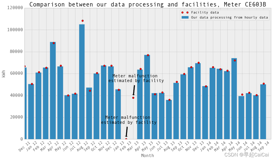
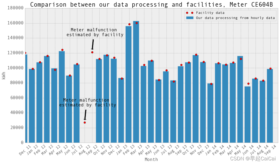
这张图片中的点是设施提供的月度数据。它们是账单上的数字。当电表发生故障时，设施会估算用电量以进行计费。我们在绘图中排除的数据点不在图中。它们的用电量远高于正常水平（比其他正常用电量高出30倍）。 “Meter malfunction, estimated by facility” 意味着在这个月，电表出现故障，这个点是设施估算的结果。

CE603B电表在2013年2月和3月发生了故障。CE604B电表在2012年8月和9月发生了故障。我们将这些月份的数据设置为np.nan，并将它们从回归中排除。再次绘制柱状图并与设施提供的月度数据进行比较。它们吻合！当然，除了电表发生故障的那些月份。在这些月份，设施估算用电量以进行计费。对于我们来说，在回归中我们只是排除了这些月份的小时和日数据点。

建筑物的总用电量是这两个电表的电量之和。为了确保准确性，我们保留了“功率”数据并将其与“能量”数据进行比较。

electricity['energy'] = electricity['Gund Bus-A EnergyReal - kWhr'] + electricity['Gund Bus-B EnergyReal - kWhr']
electricity['power'] = electricity['Gund Bus-A PowerReal - kW'] + electricity['Gund Bus-B PowerReal - kW']
electricity.head()

在这里插入图片描述

Derive hourly consumption

计算每小时用电量

计算每小时用电量的方法是，下一个小时的电表度数减去当前小时的电表度数，即"energy"列中下一个小时的数值减去当前小时的数值。我们假设电表度数是在小时结束时记录的。为了避免混淆，我们在数据框中还标记了电表读数的开始时间和结束时间。我们比较了下一个小时的功率数据和计算得到的每小时用电量，大部分情况下，功率和每小时用电量相差不大。但有时候有很大的差异。

电表记录的是累积用电量。例如，今天开始时，电表度数为10。一个小时后，用电量为1，那么电表读数就加一变为11，以此类推。因此，电表读数应该一直在增加。然而，我们发现有时电表读数会突然掉到0，然后过了一段时间后再次变成很高的正数。这会导致负的每小时用电量，然后是荒谬的极高的正数。我们通过计算t + 1时刻的电表读数 - t时刻的电表读数来获取每小时/每日的用电量。如果结果是负数或荒谬地高，我们就认为电表发生了故障。现在我们将这些数据点设置为np.nan。通过查看电子表格中的原始数据和月度绘图，我们确定了电表故障的确切日期。

此外，有时会出现比正常值高出千倍的荒谬数据点。正常的每小时用电量范围在100至400之间。我们创建了一个过滤器：index = abs(hourlyEnergy) < 200000，这意味着只有低于200000的值才会被保留。

# In case there are any missing hours, reindex to get the entire time span. Fill in nan data.
hourlyTimestamp = pd.date_range(start = '2011/7/1', end = '2014/10/31', freq = 'H')

# Somehow, reindex does not work well. October 2011 and several other hours are missing. 
# Basically it is just the length of original length.
#electricity.reindex(hourlyTimestamp, inplace = True, fill_value = np.nan)

startTime = hourlyTimestamp
endTime = hourlyTimestamp + np.timedelta64(1,'h')
hourlyTime = pd.DataFrame(data = np.transpose([startTime, endTime]), index = hourlyTimestamp, columns = ['startTime', 'endTime'])

electricity = electricity.join(hourlyTime, how = 'outer')

# Just in case, in order to use diff method, timestamp has to be in asending order.
electricity.sort_index(inplace = True)
hourlyEnergy = electricity.diff(periods=1)['energy']

hourlyElectricity = pd.DataFrame(data = hourlyEnergy.values, index = hourlyEnergy.index, columns = ['electricity-kWh'])
hourlyElectricity = hourlyElectricity.join(hourlyTime, how = 'inner')

print("Data length: ", len(hourlyElectricity)/24, " days")
hourlyElectricity.head()

这段代码的功能是将原始数据转换为每小时的用电量数据，并将其存储在名为“hourlyElectricity”的数据框中。具体来说：

首先，使用“pd.date_range”函数创建一个包含每个小时时间戳的时间序列“hourlyTimestamp”，以便在后续的操作中使用。
然后，使用“hourlyTimestamp”对数据框进行重新索引，以确保数据涵盖整个时间跨度，并使用“np.nan”填充缺失值。但是，由于重新索引存在问题，缺失的小时并没有成功填充，因此在后续操作中使用了另一种方法。
接着，创建一个名为“hourlyTime”的数据框，其中包含每个小时的开始时间和结束时间。这可以帮助我们跟踪每个小时的时间段。
使用“join”方法将“hourlyTime”数据框与“electricity”数据框合并，并使用缺失值填充任何缺失数据。
然后，将数据框按照时间戳升序排列，使用“diff”方法计算每小时的用电量，将结果存储在名为“hourlyEnergy”的数据框中。
最后，创建一个名为“hourlyElectricity”的数据框，其中包含每小时的用电量和时间戳信息，并将其与“hourlyTime”数据框合并。

代码最后输出了数据长度（即数据覆盖的天数）和前几行“hourlyElectricity”数据框的内容。

在这里插入图片描述

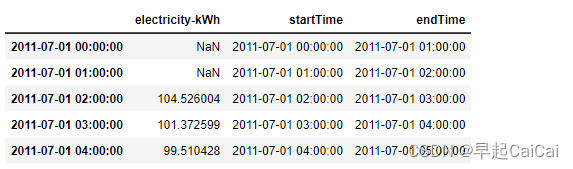
以上是每小时的用电量数据。数据被导出到一个Excel文件中。我们假设电表读数是在小时结束时记录的。

# Filter the data, keep the NaN and generate two excels, with and without Nan

hourlyElectricity.loc[abs(hourlyElectricity['electricity-kWh']) > 100000,'electricity-kWh'] = np.nan

time = hourlyElectricity.index
index = ((time > np.datetime64('2012-07-26')) & (time < np.datetime64('2012-08-18'))) \
        | ((time > np.datetime64('2013-01-21')) & (time < np.datetime64('2013-03-08')))

hourlyElectricity.loc[index,'electricity-kWh'] = np.nan
hourlyElectricityWithoutNaN = hourlyElectricity.dropna(axis=0, how='any')

hourlyElectricity.to_excel('Data/hourlyElectricity.xlsx')
hourlyElectricityWithoutNaN.to_excel('Data/hourlyElectricityWithoutNaN.xlsx')

这段代码的功能是过滤数据，保留NaN，并分别生成两个Excel文件，一个包含NaN，一个不包含NaN。

具体来说：

首先，使用“loc”函数根据每小时用电量的绝对值是否大于100000来过滤数据，将超过该阈值的数据设置为NaN。
然后，创建一个名为“index”的布尔索引，根据时间戳选择数据，将指定时间范围内的数据设置为NaN。
接着，使用“dropna”函数删除任何包含NaN的行，并将结果存储在名为“hourlyElectricityWithoutNaN”的数据框中。
最后，使用“to_excel”函数将包含NaN的数据框“hourlyElectricity”和不包含NaN的数据框“hourlyElectricityWithoutNaN”分别导出到两个Excel文件中。

该代码的输出是两个Excel文件，分别为“hourlyElectricity.xlsx”和“hourlyElectricityWithoutNaN.xlsx”，用于进一步分析和处理数据。

plt.figure()
fig = hourlyElectricity.plot(fontsize = 15, figsize = (15, 6))
plt.tick_params(which=u'major', reset=False, axis = 'y', labelsize = 15)
fig.set_axis_bgcolor('w')
plt.title('All the hourly electricity data', fontsize = 16)
plt.ylabel('kWh')
plt.show()

plt.figure()
fig = hourlyElectricity.iloc[26200:27400,:].plot(marker = 'o',label='hourly electricity', fontsize = 15, figsize = (15, 6))
plt.tick_params(which=u'major', reset=False, axis = 'y', labelsize = 15)
fig.set_axis_bgcolor('w')
plt.title('Hourly electricity data of selected days', fontsize = 16)
plt.ylabel('kWh')
plt.legend()
plt.show()

在这里插入图片描述

以上是每小时数据的图表。在第一个图表中，空缺的部分是由于电表故障时导致的数据缺失。在第二个图表中，您可以看到白天和晚上、工作日和周末之间的差异。

Derive daily consumption

计算每天消耗量

我们通过“reindex”成功获取了每日的电力消耗量。

dailyTimestamp = pd.date_range(start = '2011/7/1', end = '2014/10/31', freq = 'D')
electricityReindexed = electricity.reindex(dailyTimestamp, inplace = False)

# Just in case, in order to use diff method, timestamp has to be in asending order.
electricityReindexed.sort_index(inplace = True)
dailyEnergy = electricityReindexed.diff(periods=1)['energy']

dailyElectricity = pd.DataFrame(data = dailyEnergy.values, index = electricityReindexed.index - np.timedelta64(1,'D'), columns = ['electricity-kWh'])
dailyElectricity['startDay'] = dailyElectricity.index
dailyElectricity['endDay'] = dailyElectricity.index + np.timedelta64(1,'D')

# Filter the data, keep the NaN and generate two excels, with and without Nan

dailyElectricity.loc[abs(dailyElectricity['electricity-kWh']) > 2000000,'electricity-kWh'] = np.nan

time = dailyElectricity.index
index = ((time > np.datetime64('2012-07-26')) & (time < np.datetime64('2012-08-18'))) | ((time > np.datetime64('2013-01-21')) & (time < np.datetime64('2013-03-08')))

dailyElectricity.loc[index,'electricity-kWh'] = np.nan
dailyElectricityWithoutNaN = dailyElectricity.dropna(axis=0, how='any')

dailyElectricity.to_excel('Data/dailyElectricity.xlsx')
dailyElectricityWithoutNaN.to_excel('Data/dailyElectricityWithoutNaN.xlsx')

dailyElectricity.head()

代码解释：

dailyTimestamp = pd.date_range(start='2011/7/1', end='2014/10/31', freq='D'): 创建一个日期范围，从2011年7月1日到2014年10月31日，以每日为频率。
electricityReindexed = electricity.reindex(dailyTimestamp, inplace=False): 使用"reindex"方法将原始数据集重新索引为每日的时间戳，生成一个新的DataFrame对象。
electricityReindexed.sort_index(inplace=True): 确保时间戳按升序排序，以便后续使用"diff"方法。
dailyEnergy = electricityReindexed.diff(periods=1)['energy']: 使用"diff"方法计算每日能量消耗量的差异，并将结果存储在"dailyEnergy"列中。
dailyElectricity = pd.DataFrame(data=dailyEnergy.values, index=electricityReindexed.index - np.timedelta64(1, 'D'), columns=['electricity-kWh']): 创建一个新的DataFrame对象"dailyElectricity"，其中包含每日电力消耗量和起始日期。
dailyElectricity['startDay'] = dailyElectricity.index: 添加一个"startDay"列，包含每日消耗量的起始日期。
dailyElectricity['endDay'] = dailyElectricity.index + np.timedelta64(1, 'D'): 添加一个"endDay"列，包含每日消耗量的结束日期。
dailyElectricity.loc[abs(dailyElectricity['electricity-kWh']) > 2000000, 'electricity-kWh'] = np.nan: 将电力消耗量超过2000000的值设为NaN（缺失值）。
time = dailyElectricity.index: 获取每日消耗量的时间索引。
index = ((time > np.datetime64('2012-07-26')) & (time < np.datetime64('2012-08-18'))) | ((time > np.datetime64('2013-01-21')) & (time < np.datetime64('2013-03-08'))): 创建一个布尔索引，用于筛选出指定时间范围内的数据。
dailyElectricity.loc[index, 'electricity-kWh'] = np.nan: 将指定时间范围内的电力消耗量设为NaN。
dailyElectricityWithoutNaN = dailyElectricity.dropna(axis=0, how='any'): 创建一个新的DataFrame对象"dailyElectricityWithoutNaN"，删除包含NaN值的行。
dailyElectricity.to_excel('Data/dailyElectricity.xlsx'): 将"dailyElectricity"保存为Excel文件。
dailyElectricityWithoutNaN.to_excel('Data/dailyElectricityWithoutNaN.xlsx'): 将"dailyElectricityWithoutNaN"保存为Excel文件。
dailyElectricity.head(): 显示"dailyElectricity"的前几行数据。

在这里插入图片描述

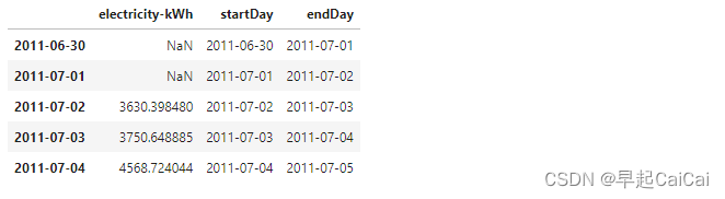
Above is the daily electricity consumption.

plt.figure()
fig = dailyElectricity.plot(figsize = (15, 6))
fig.set_axis_bgcolor('w')
plt.title('All the daily electricity data', fontsize = 16)
plt.ylabel('kWh')
plt.show()

plt.figure()
fig = dailyElectricity.iloc[1000:1130,:].plot(marker = 'o', figsize = (15, 6))
fig.set_axis_bgcolor('w')
plt.title('Daily electricity data of selected days', fontsize = 16)
plt.ylabel('kWh')
plt.show()

在这里插入图片描述

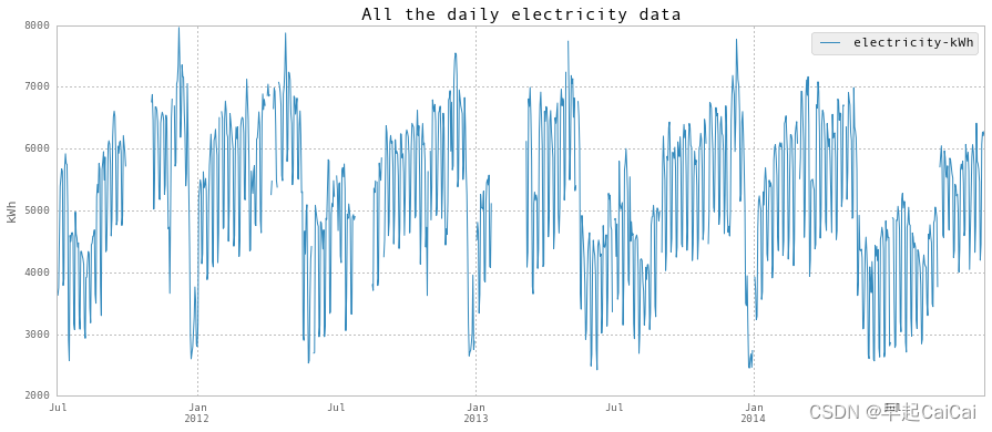
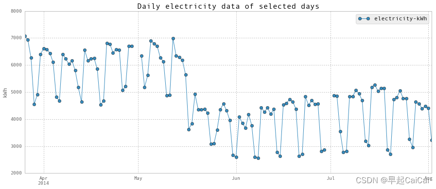
Above is the daily electricity plot.
超低的电力消耗发生在学期结束后，包括圣诞假期。此外，正如您在第二个图表中所看到的，夏季开始上学后能源消耗较低。

Chilled Water

冷水
We clean the chilled water data in the same way as electricity.

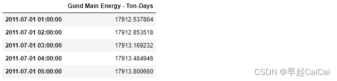
chilledWater = df[['Gund Main Energy - Ton-Days']]
chilledWater.head()

在这里插入图片描述

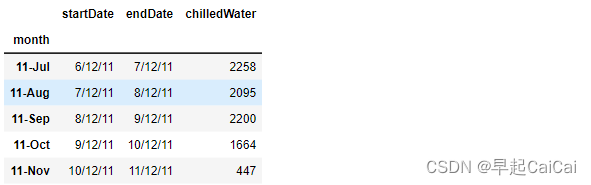
file = 'Data/monthly chilled water.csv' 
monthlyChilledWaterFromFacility = pd.read_csv(file, header=0)
monthlyChilledWaterFromFacility.set_index(['month'], inplace = True)
monthlyChilledWaterFromFacility.head()

在这里插入图片描述

monthlyChilledWaterFromFacility['startDate'] = pd.to_datetime(monthlyChilledWaterFromFacility['startDate'], format="%m/%d/%y")
values = monthlyChilledWaterFromFacility.index.values

keys = np.array(monthlyChilledWaterFromFacility['startDate'])

dates = {}
for key, value in zip(keys, values):
    dates[key] = value

sortedDates =  np.sort(dates.keys())
sortedDates = sortedDates[sortedDates > np.datetime64('2011-11-01')]

months = []
monthlyChilledWaterOrg = np.zeros((len(sortedDates) - 1))
for i in range(len(sortedDates) - 1):
    begin = sortedDates[i]
    end = sortedDates[i+1]
    months.append(dates[sortedDates[i]])
    monthlyChilledWaterOrg[i] = (np.round(chilledWater.loc[end,:] -  chilledWater.loc[begin,:], 1))
    

monthlyChilledWater = pd.DataFrame(data = monthlyChilledWaterOrg, index = months, columns = ['chilledWater-TonDays'])

fig,ax = plt.subplots(1, 1,figsize=(15,8))
#ax.set_axis_bgcolor('w')
#plt.plot(monthlyChilledWater, label='Our data processing from hourly data', marker = 'x', markersize = 15, linestyle = '')
plt.bar(np.arange(len(monthlyChilledWater))-0.5, monthlyChilledWater.values, label='Our data processing from hourly data')
plt.plot(monthlyChilledWaterFromFacility[5:-1]['chilledWater'],'or', label='Facility data')
plt.xticks(np.arange(0,len(months)),months)
plt.xlabel('Month',fontsize=15)
plt.ylabel('kWh',fontsize=15)
plt.xlim([0,len(months)])
plt.legend()
ax.set_xticklabels(months, rotation=40, fontsize=13)
plt.tick_params(which=u'major', reset=False, axis = 'y', labelsize = 15)
plt.title('Data Validation: comparison between our data processing and facilities',fontsize=20)

text = 'Match! Our processing method is valid.'
ax.annotate(text, xy = (15, 2000), 
            xytext = (5, 50), fontsize = 15, 
            textcoords = 'offset points', ha = 'center', va = 'bottom')

plt.show()

代码的解释如下：

首先，通过pd.to_datetime将monthlyChilledWaterFromFacility中的日期列转换为datetime格式。

然后，从monthlyChilledWaterFromFacility获取索引的值，并将其存储在values中。

接下来，将monthlyChilledWaterFromFacility中的开始日期列存储在keys中。

通过循环遍历keys和values，将日期和索引值存储在dates字典中。

对dates字典的键进行排序，并将排序后的日期存储在sortedDates中。然后，从sortedDates中筛选出大于指定日期的日期。

创建空列表months，用于存储月份。

使用np.zeros创建一个长度为sortedDates减1的零数组monthlyChilledWaterOrg。

通过循环遍历sortedDates，计算每个月的冷水消耗量，并将结果存储在monthlyChilledWaterOrg中。

将monthlyChilledWaterOrg转换为DataFrame，使用months作为索引，列名为chilledWater-TonDays。

创建一个图表，并使用plt.bar绘制我们从小时数据处理得到的冷水消耗量，使用plt.plot绘制设备数据。

在这里插入图片描述

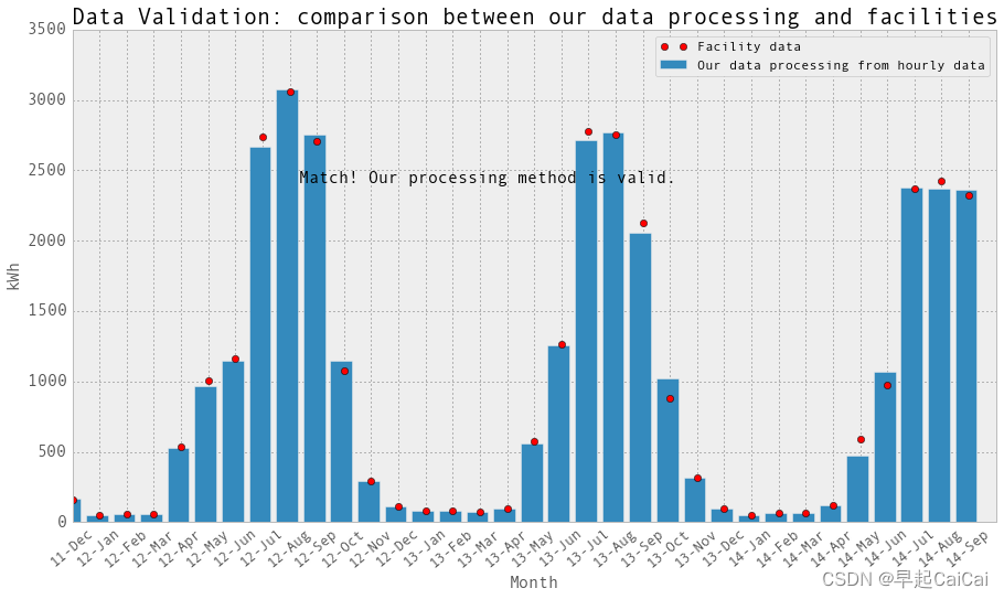
上图中红点为设施的数据，bar为我们从每小时数据获取的每天的数据，两者基本一致，说明我们处理的方法是正确的

hourlyTimestamp = pd.date_range(start = '2011/7/1', end = '2014/10/31', freq = 'H')
chilledWater.reindex(hourlyTimestamp, inplace = True)

# Just in case, in order to use diff method, timestamp has to be in asending order.
chilledWater.sort_index(inplace = True)
hourlyEnergy = chilledWater.diff(periods=1)

hourlyChilledWater = pd.DataFrame(data = hourlyEnergy.values, index = hourlyEnergy.index, columns = ['chilledWater-TonDays'])
hourlyChilledWater['startTime'] = hourlyChilledWater.index
hourlyChilledWater['endTime'] = hourlyChilledWater.index + np.timedelta64(1,'h')

hourlyChilledWater.loc[abs(hourlyChilledWater['chilledWater-TonDays']) > 50,'chilledWater-TonDays'] = np.nan

hourlyChilledWaterWithoutNaN = hourlyChilledWater.dropna(axis=0, how='any')

hourlyChilledWater.to_excel('Data/hourlyChilledWater.xlsx')
hourlyChilledWaterWithoutNaN.to_excel('Data/hourlyChilledWaterWithoutNaN.xlsx')

plt.figure()
fig = hourlyChilledWater.plot(fontsize = 15, figsize = (15, 6))
plt.tick_params(which=u'major', reset=False, axis = 'y', labelsize = 15)
fig.set_axis_bgcolor('w')
plt.title('All the hourly chilled water data', fontsize = 16)
plt.ylabel('Ton-Days')
plt.show()

hourlyChilledWater.head()

代码的解释如下：

首先，使用pd.date_range生成从开始日期到结束日期的逐小时时间戳，存储在hourlyTimestamp中。

通过reindex方法，将冷水数据重新索引为逐小时时间戳，并将结果存储在chilledWater中。

接下来，对chilledWater进行按索引排序，以确保时间戳按升序排列。

使用diff方法计算每小时的冷水消耗量，并将结果存储在hourlyEnergy中。

创建一个DataFrame，使用hourlyEnergy的值作为数据，时间戳作为索引，列名为chilledWater-TonDays。

添加startTime和endTime列，分别表示每小时的起始时间和结束时间。

通过loc方法，将冷水消耗量绝对值大于50的数据设置为NaN。

使用dropna方法删除含有NaN值的行，并将结果存储在hourlyChilledWaterWithoutNaN中。

将hourlyChilledWater和hourlyChilledWaterWithoutNaN分别保存为Excel文件。

创建一个图表，并使用plot方法绘制所有小时级冷水数据。

在这里插入图片描述

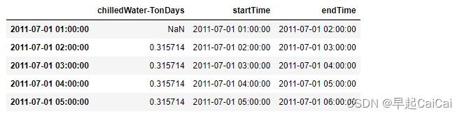
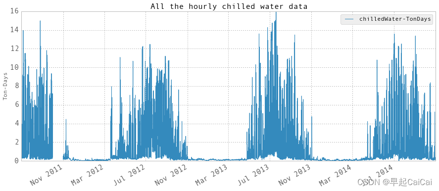
上图为hourlyEnergy的值

dailyTimestamp = pd.date_range(start = '2011/7/1', end = '2014/10/31', freq = 'D')
chilledWaterReindexed = chilledWater.reindex(dailyTimestamp, inplace = False)

chilledWaterReindexed.sort_index(inplace = True)
dailyEnergy = chilledWaterReindexed.diff(periods=1)['Gund Main Energy - Ton-Days']

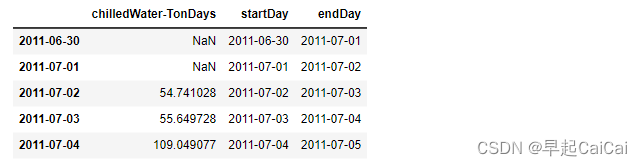
dailyChilledWater = pd.DataFrame(data = dailyEnergy.values, index = chilledWaterReindexed.index - np.timedelta64(1,'D'), columns = ['chilledWater-TonDays'])
dailyChilledWater['startDay'] = dailyChilledWater.index
dailyChilledWater['endDay'] = dailyChilledWater.index + np.timedelta64(1,'D')

dailyChilledWaterWithoutNaN = dailyChilledWater.dropna(axis=0, how='any')

dailyChilledWater.to_excel('Data/dailyChilledWater.xlsx')
dailyChilledWaterWithoutNaN.to_excel('Data/dailyChilledWaterWithoutNaN.xlsx')

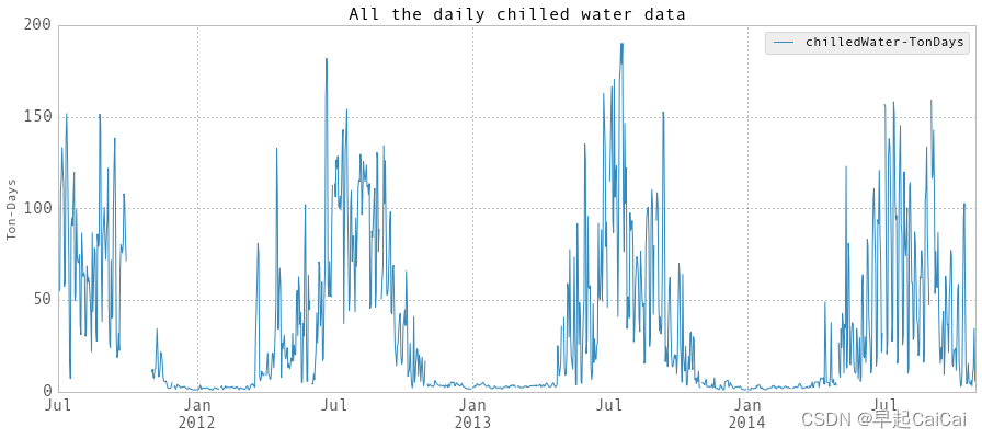
plt.figure()
fig = dailyChilledWater.plot(fontsize = 15, figsize = (15, 6))
plt.tick_params(which=u'major', reset=False, axis = 'y', labelsize = 15)
fig.set_axis_bgcolor('w')
plt.title('All the daily chilled water data', fontsize = 16)
plt.ylabel('Ton-Days')
plt.show()


dailyChilledWater.head()

代码的解释如下：

首先，使用pd.date_range生成从开始日期到结束日期的逐日时间戳，存储在dailyTimestamp中。

通过reindex方法，将冷水数据重新索引为逐日时间戳，并将结果存储在chilledWaterReindexed中。

接下来，对chilledWaterReindexed进行按索引排序，以确保时间戳按升序排列。

使用diff方法计算每天的冷水消耗量，并将结果存储在dailyEnergy中，列名为’Gund Main Energy - Ton-Days’。

创建一个DataFrame，使用dailyEnergy的值作为数据，时间戳减去1天作为索引，列名为chilledWater-TonDays。

添加startDay和endDay列，分别表示每天的起始时间和结束时间。

使用dropna方法删除含有NaN值的行，并将结果存储在dailyChilledWaterWithoutNaN中。

将dailyChilledWater和dailyChilledWaterWithoutNaN分别保存为Excel文件。

创建一个图表，并使用plot方法绘制所有每日级冷水数据。

在这里插入图片描述

Steam

蒸汽

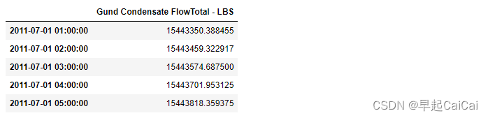
steam = df[['Gund Condensate FlowTotal - LBS']]
steam.head()

在这里插入图片描述

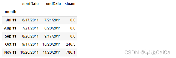
file = 'Data/monthly steam.csv' 
monthlySteamFromFacility = pd.read_csv(file, header=0)
monthlySteamFromFacility.set_index(['month'], inplace = True)
monthlySteamFromFacility.head()

在这里插入图片描述

monthlySteamFromFacility['startDate'] = pd.to_datetime(monthlySteamFromFacility['startDate'], format="%m/%d/%Y")
values = monthlySteamFromFacility.index.values

keys = np.array(monthlySteamFromFacility['startDate'])

dates = {}
for key, value in zip(keys, values):
    dates[key] = value

sortedDates =  np.sort(dates.keys())
sortedDates = sortedDates[sortedDates > np.datetime64('2011-11-01')]

months = []
monthlySteamOrg = np.zeros((len(sortedDates) - 1))
for i in range(len(sortedDates) - 1):
    begin = sortedDates[i]
    end = sortedDates[i+1]
    months.append(dates[sortedDates[i]])
    monthlySteamOrg[i] = (np.round(steam.loc[end,:] -  steam.loc[begin,:], 1))
    

monthlySteam = pd.DataFrame(data = monthlySteamOrg, index = months, columns = ['steam-LBS'])

# 867 LBS ~= 1MMBTU steam

fig,ax = plt.subplots(1, 1,figsize=(15,8))
#ax.set_axis_bgcolor('w')
#plt.plot(monthlySteam/867, label='Our data processing from hourly data')
plt.bar(np.arange(len(monthlySteam))-0.5, monthlySteam.values/867, label='Our data processing from hourly data')
plt.plot(monthlySteamFromFacility.loc[months,'steam'],'or', label='Facility data')
plt.xticks(np.arange(0,len(months)),months)
plt.xlabel('Month',fontsize=15)
plt.ylabel('Steam (MMBTU)',fontsize=15)
plt.xlim([0,len(months)])
plt.legend()
ax.set_xticklabels(months, rotation=40, fontsize=13)
plt.tick_params(which=u'major', reset=False, axis = 'y', labelsize = 15)
plt.title('Comparison between our data processing and facilities - Steam',fontsize=20)

text = 'Match! Our processing method is valid.'
ax.annotate(text, xy = (9, 1500), 
            xytext = (5, 50), fontsize = 15, 
            textcoords = 'offset points', ha = 'center', va = 'bottom')

plt.show()

代码的解释如下：

首先，将monthlySteamFromFacility中的"startDate"列转换为日期时间格式，格式为"%m/%d/%Y"，并将结果存储在该列中。

将monthlySteamFromFacility的索引值存储在values中。

创建一个keys数组，其中存储了monthlySteamFromFacility的"startDate"列的值。

创建一个空字典dates，用于存储"startDate"和索引值之间的映射关系。

使用zip函数将keys和values进行迭代，将"startDate"和索引值存储在dates字典中。

对dates.keys()进行排序，将结果存储在sortedDates中。

从sortedDates中选择大于日期'2011-11-01'的日期，并重新赋值给sortedDates。

创建一个空列表months，用于存储每个时间段的月份。

创建一个长度为len(sortedDates) - 1的零数组monthlySteamOrg。

使用循环遍历sortedDates中的日期，并根据日期计算每个时间段的蒸汽消耗量。

将对应的月份添加到months列表中。

将计算得到的蒸汽消耗量存储在monthlySteamOrg数组中。

创建一个DataFrame，使用monthlySteamOrg的值作为数据，months作为索引，列名为"steam-LBS"。

创建一个图表，并使用bar和plot方法分别绘制我们的数据处理结果和设施数据的对比。

在这里插入图片描述

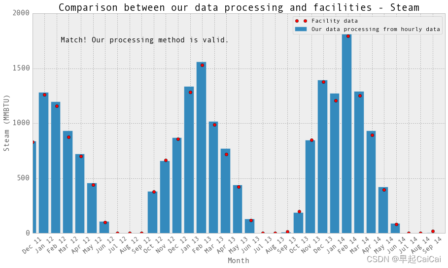
我们的处理数据与设备的数据是一致的

和上面一样：绘制出 hourly steam data; daily steam data

hourlyTimestamp = pd.date_range(start = '2011/7/1', end = '2014/10/31', freq = 'H')
steam.reindex(hourlyTimestamp, inplace = True)

# Just in case, in order to use diff method, timestamp has to be in asending order.
steam.sort_index(inplace = True)
hourlyEnergy = steam.diff(periods=1)

hourlySteam = pd.DataFrame(data = hourlyEnergy.values, index = hourlyEnergy.index, columns = ['steam-LBS'])
hourlySteam['startTime'] = hourlySteam.index
hourlySteam['endTime'] = hourlySteam.index + np.timedelta64(1,'h')

hourlySteam.loc[abs(hourlySteam['steam-LBS']) > 100000,'steam-LBS'] = np.nan

plt.figure()
fig = hourlySteam.plot(fontsize = 15, figsize = (15, 6))
plt.tick_params(which=u'major', reset=False, axis = 'y', labelsize = 17)
fig.set_axis_bgcolor('w')
plt.title('All the hourly steam data', fontsize = 16)
plt.ylabel('LBS')
plt.show()

hourlySteamWithoutNaN = hourlySteam.dropna(axis=0, how='any')

hourlySteam.to_excel('Data/hourlySteam.xlsx')
hourlySteamWithoutNaN.to_excel('Data/hourlySteamWithoutNaN.xlsx')

hourlySteam.head()

在这里插入图片描述

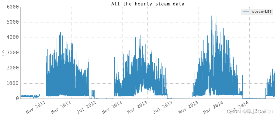
hourly steam data

dailyTimestamp = pd.date_range(start = '2011/7/1', end = '2014/10/31', freq = 'D')
steamReindexed = steam.reindex(dailyTimestamp, inplace = False)

steamReindexed.sort_index(inplace = True)
dailyEnergy = steamReindexed.diff(periods=1)['Gund Condensate FlowTotal - LBS']

dailySteam = pd.DataFrame(data = dailyEnergy.values, index = steamReindexed.index - np.timedelta64(1,'D'), columns = ['steam-LBS'])
dailySteam['startDay'] = dailySteam.index
dailySteam['endDay'] = dailySteam.index + np.timedelta64(1,'D')

plt.figure()
fig = dailySteam.plot(fontsize = 15, figsize = (15, 6))
plt.tick_params(which=u'major', reset=False, axis = 'y', labelsize = 15)
fig.set_axis_bgcolor('w')
plt.title('All the daily steam data', fontsize = 16)
plt.ylabel('LBS')
plt.show()

dailySteamWithoutNaN = dailyChilledWater.dropna(axis=0, how='any')

dailySteam.to_excel('Data/dailySteam.xlsx')
dailySteamWithoutNaN.to_excel('Data/dailySteamWithoutNaN.xlsx')

dailySteam.head()

在这里插入图片描述

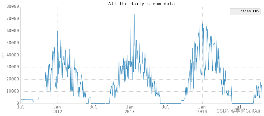
daily steam data

Reference

cs109-energy+哈佛大学能源探索项目 Part-1（项目背景）
一个完整的机器学习项目实战代码+数据分析过程：哈佛大学能耗预测项目
Part 1-3 Project Overview, Data Wrangling and Exploratory Analysis-DEC10
Prediction of Buildings Energy Consumption