来源:《斯坦福数据挖掘教程·第三版》对应的公开英文书和PPT
Chapter 6 Frequent Itemsets
The market-basket model of data is used to describe a common form of many-many relationship between two kinds of objects. On the one hand, we have items, and on the other we have baskets, sometimes called “transactions.” Each basket consists of a set of items (an itemset), and usually we assume that the number of items in a basket is small – much smaller than the total number of items. The number of baskets is usually assumed to be very large, bigger than what can fit in main memory. The data is assumed to be represented in a file consisting of a sequence of baskets. In terms of the distributed file system, the baskets are the objects of the file, and each basket is of type “set of items.”
We assume there is a number s, called the support threshold. If I is a set of items, the support for I is the number of baskets for which I is a subset. We say I is frequent if its support is s or more.
Suppose that we set our threshold at s = 3 s = 3 s=3. Then there are five frequent singleton itemsets: {dog}, {cat}, {and}, {a}, and {training}.
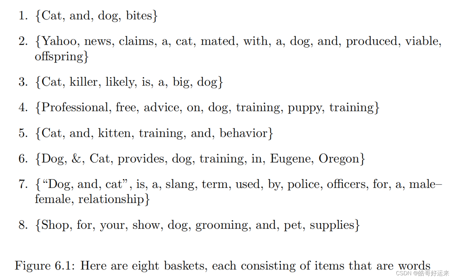
A doubleton cannot be frequent unless both items in the set are frequent by themselves.
Applications of frequent-itemset analysis is not limited to market baskets. The same model can be used to mine many other kinds of data. Some examples are:
- Related concepts: Let items be words, and let baskets be documents. A basket/document contains those items/words that are present in the document. If we look for sets of words that appear together in many documents, the sets will be dominated by the most common words (stop words). There, even though the intent was to find snippets that talked about cats and dogs, the stop words “and” and “a” were prominent among the frequent itemsets. However, if we ignore all the most common words, then we would hope to find among the frequent pairs some pairs of words that represent a joint concept.
- Plagiarism: Let the items be documents and the baskets be sentences. An item/document is “in” a basket/sentence if the sentence is in the document. This arrangement appears backwards, but it is exactly what we need, and we should remember that the relationship between items and baskets is an arbitrary many-many relationship. That is, “in” need not have its conventional meaning: “part of.” In this application, we look for pairs of items that appear together in several baskets. If we find such a pair, then we have two documents that share several sentences in common. In practice, even one or two sentences in common is a good indicator of plagiarism.
- Biomarkers: Let the items be of two types – biomarkers such as genes or blood proteins, and diseases. Each basket is the set of data about a patient: their genome and blood-chemistry analysis, as well as their medical history of disease. A frequent itemset that consists of one disease and one or more biomarkers suggests a test for the disease.
Thus, we define the interest of an association rule I → j I → j I→j to be the difference between its confidence and the fraction of baskets that contain j.
There is another approach to storing counts that may be more appropriate, depending on the fraction of the possible pairs of items that actually appear in some basket. We can store counts as triples [ i , j , c ] [i, j, c] [i,j,c], meaning that the count of pair { i , j } \{i, j\} {i,j}, with i < j i < j i<j, is c c c. A data structure, such as a hash table with i i i and j j j as the search key, is used so we can tell if there is a triple for a given i i i and j j j and, if so, to find it quickly. We call this approach the triples method of storing counts.
the A-Priori Algorithm, one pass is taken for each set-size k. If no frequent itemsets of a certain size are found, then monotonicity tells us there can be no larger frequent itemsets, so we can stop.
The pattern of moving from one size k to the next size k + 1 k + 1 k+1 can be summarized as follows. For each size k, there are two sets of itemsets:
- C k C_k Ck is the set of candidate itemsets of size k – the itemsets that we must count in order to determine whether they are in fact frequent.
- L k L_k Lk is the set of truly frequent itemsets of size k k k. The pattern of moving from one set to the next and one size to the next is suggested by Fig. 6.4.

Summary of Chapter 6
- Market-Basket Data: This model of data assumes there are two kinds of entities: items and baskets. There is a many–many relationship between items and baskets. Typically, baskets are related to small sets of items, while items may be related to many baskets.
- Frequent Itemsets: The support for a set of items is the number of baskets containing all those items. Itemsets with support that is at least some threshold are called frequent itemsets.
- Association Rules: These are implications that if a basket contains a certain set of items I, then it is likely to contain another particular item j as well. The probability that j is also in a basket containing I is called the confidence of the rule. The interest of the rule is the amount by which the confidence deviates from the fraction of all baskets that contain j.
- The Pair-Counting Bottleneck: To find frequent itemsets, we need to examine all baskets and count the number of occurrences of sets of a certain size. For typical data, with a goal of producing a small number of itemsets that are the most frequent of all, the part that often takes the most main memory is the counting of pairs of items. Thus, methods for finding frequent itemsets typically concentrate on how to minimize the main memory needed to count pairs.
- Triangular Matrices: While one could use a two-dimensional array to count pairs, doing so wastes half the space, because there is no need to count pair { i , j } \{i, j\} {i,j} in both the i-j and j-i array elements. By arranging the pairs ( i , j ) (i, j) (i,j) for which i < j i < j i<j in lexicographic order, we can store only the needed counts in a one-dimensional array with no wasted space, and yet be able to access the count for any pair efficiently.
- Storage of Pair Counts as Triples: If fewer than 1/3 of the possible pairs actually occur in baskets, then it is more space-efficient to store counts of pairs as triples ( i , j , c ) (i, j, c) (i,j,c), where c is the count of the pair { i , j } \{i, j\} {i,j}, and i < j i < j i<j. An index structure such as a hash table allows us to find the triple for ( i , j ) (i, j) (i,j) efficiently.
- Monotonicity of Frequent Itemsets: An important property of itemsets is that if a set of items is frequent, then so are all its subsets. We exploit this property to eliminate the need to count certain itemsets by using its contrapositive: if an itemset is not frequent, then neither are its supersets.
- The A-Priori Algorithm for Pairs: We can find all frequent pairs by making two passes over the baskets. On the first pass, we count the items themselves, and then determine which items are frequent. On the second pass, we count only the pairs of items both of which are found frequent on the first pass. Monotonicity justifies our ignoring other pairs.
- Finding Larger Frequent Itemsets: A-Priori and many other algorithms allow us to find frequent itemsets larger than pairs, if we make one pass over the baskets for each size itemset, up to some limit. To find the frequent itemsets of size k, monotonicity lets us restrict our attention to only those itemsets such that all their subsets of size k − 1 k − 1 k−1 have already been found frequent.
- The PCY Algorithm: This algorithm improves on A-Priori by creating a hash table on the first pass, using all main-memory space that is not needed to count the items. Pairs of items are hashed, and the hash-table buckets are used as integer counts of the number of times a pair has hashed to that bucket. Then, on the second pass, we only have to count pairs of frequent items that hashed to a frequent bucket (one whose count is at least the support threshold) on the first pass.
- The Multistage Algorithm: We can insert additional passes between the first and second pass of the PCY Algorithm to hash pairs to other, independent hash tables. At each intermediate pass, we only have to hash pairs of frequent items that have hashed to frequent buckets on all previous passes.
- The Multihash Algorithm: We can modify the first pass of the PCY Algorithm to divide available main memory into several hash tables. On the second pass, we only have to count a pair of frequent items if they hashed to frequent buckets in all hash tables.
- Randomized Algorithms: Instead of making passes through all the data, we may choose a random sample of the baskets, small enough that it is possible to store both the sample and the needed counts of itemsets in main memory. The support threshold must be scaled down in proportion. We can then find the frequent itemsets for the sample, and hope that it is a good representation of the data as whole. While this method uses at most one pass through the whole dataset, it is subject to false positives (itemsets that are frequent in the sample but not the whole) and false negatives (itemsets that are frequent in the whole but not the sample).
- The SON Algorithm: An improvement on the simple randomized algorithm is to divide the entire file of baskets into segments small enough that all frequent itemsets for the segment can be found in main memory. Candidate itemsets are those found frequent for at least one segment. A second pass allows us to count all the candidates and find the exact collection of frequent itemsets. This algorithm is especially appropriate in a
MapReduce setting. - Toivonen’s Algorithm: This algorithm starts by finding frequent itemsets in a sample, but with the threshold lowered so there is little chance of missing an itemset that is frequent in the whole. Next, we examine the entire file of baskets, counting not only the itemsets that are frequent in the sample, but also, the negative border – itemsets that have not been found frequent, but all their immediate subsets are. If no member of the
negative border is found frequent in the whole, then the answer is exact. But if a member of the negative border is found frequent, then the whole process has to repeat with another sample. - Frequent Itemsets in Streams: If we use a decaying window with constant c c c, then we can start counting an item whenever we see it in a basket. We start counting an itemset if we see it contained within the current basket, and all its immediate proper subsets already are being counted. As the window is decaying, we multiply all counts by 1 − c 1 − c 1−c and eliminate those that are less than 1 / 2 1/2 1/2.
END

