brief

• seurat提供的教学里面包含了Standard pre-processing workflow,workflow包括QC，normalization，scale data ，detection of highly variable features。
• 其中 normalization就有蛮多方法的，seurat自己就提供了两种，一种是"LogNormalization"，另一种是目前正在大力推荐的"SCTransform",而且每一种方法参数众多，我觉得有必要对其进行仔细的探究，所以需要分开学习和记录。
• 还有 detection of highly variable features以及scale data，也是方法和参数众多，我觉得有必要对其进行仔细的探究，所以需要分开学习和记录
• • 概要图以及系列博文可以参见链接。
    
    这里主要记录了Normalize Data的学习过程，包括LogNormalization 和 SCTransform两种normalization方法的参数以及对数据的影响，以及对下游数据处理流程的影响等。

实例

Normalization之前的预处理

library(dplyr)
library(Seurat)
library(patchwork)

rm(list=ls())

# 使用read10X读取output of the cellranger pipeline from 10X，包括barcodes，genes，matrix.mtx三个文件
pbmc.data <- Read10X(data.dir = "D:/djs/pbmc3k_filtered_gene_bc_matrices/filtered_gene_bc_matrices/hg19")
# 使用 CreateSeuratObject函数构造seurat对象
pbmc <- CreateSeuratObject(counts = pbmc.data, project = "pbmc3k",
                           min.cells = 3, min.features = 200,
                           names.delim = "-",names.field = 1)

pbmc[["percent.mt"]] <- PercentageFeatureSet(pbmc, pattern = "^MT-")

pbmc <- subset(pbmc, subset = nFeature_RNA > 200 & nFeature_RNA < 2500 & percent.mt < 5)

NormalizeData --> LogNormalize

• object
  上述构建的seurat object

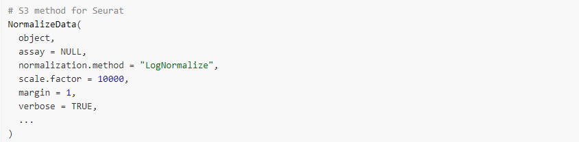
• normalization.method

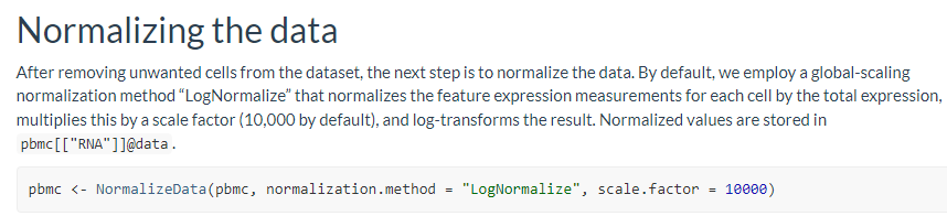
  • LogNormalize: Feature counts for each cell are divided by the total counts for that cell and multiplied by the scale.factor. This is then natural-log transformed using log1p.For counts per million (CPM) set scale.factor = 1e6

  • CLR: Applies a centered log ratio transformation

  • RC: Relative counts. Feature counts for each cell are divided by the total counts for that cell and multiplied by the scale.factor. No log-transformation is applied.

• scale.factor
  Sets the scale factor for cell-level normalization。For counts per million (CPM) set scale.factor = 1e6

• margin
  If performing CLR normalization, normalize across features (1) or cells (2)

• verbose
  display progress bar for normalization procedure

# 下面就可以进行LogNormalize
pbmc <- NormalizeData(pbmc, normalization.method = "LogNormalize", scale.factor = 10000)
# 其中NormalizeData函数提供了三个normalization.method：LogNormalize，CLR，RC，从描述可以看出来差异，那具体差在哪儿呢？

首先RC这种normalization.method我们就不考虑了，和LogNormalize比较你可以发现LogNormalize 之前做的就是RC然后做了log转化。log转化让方差稳定而且非正态的数据近似于正态分布了。
最主要要比较的是CLR和LogNormalize，CLR称为中心对数转化，具体原理和算法需要技术文档帮助，这里不写了。

# install.packages("compositions")
# library(compositions)
# library(reshape2)

pbmc_logN <- NormalizeData(pbmc, normalization.method = "LogNormalize", scale.factor = 10000)
pbmc_CLR <- NormalizeData(pbmc, normalization.method = "CLR",margin = 1)

opar <- par(no.readonly=TRUE)
par(mfrow=c(1,2))
hist(pbmc_logN[["RNA"]]@data["MT-ND4",],main = "LogNormalize",xlab = "")
hist(pbmc_CLR[["RNA"]]@data["MT-ND4",],main = "CLR",xlab = "")
par(opar)

# log转化让方差稳定而且非正态的数据近似于正态分布了,其中LogNormalize方法貌似更胜一筹
# 其中library(compositions)中有clr函数，利用clr手动处理和NormalizeData(pbmc, normalization.method = "CLR",margin = 1)
# 结果不一样

SCTransform

我目前在seurat看到的技术文档版本是V2，链接如下：
https://satijalab.org/seurat/articles/sctransform_v2_vignette.html

# install glmGamPoi,可以提高scTransform的运算速度
if (!requireNamespace("BiocManager", quietly = TRUE)) install.packages("BiocManager")
BiocManager::install("glmGamPoi")

# install sctransform >= 0.3.3
install.packages("sctransform")

library(sctransform)
# invoke sctransform - requires Seurat>=4.1
pbmc_scT <- SCTransform(pbmc, vst.flavor = "v2")
# 上面那一步就把normalization做完了

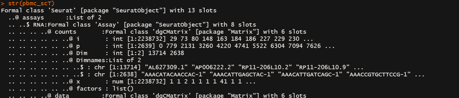
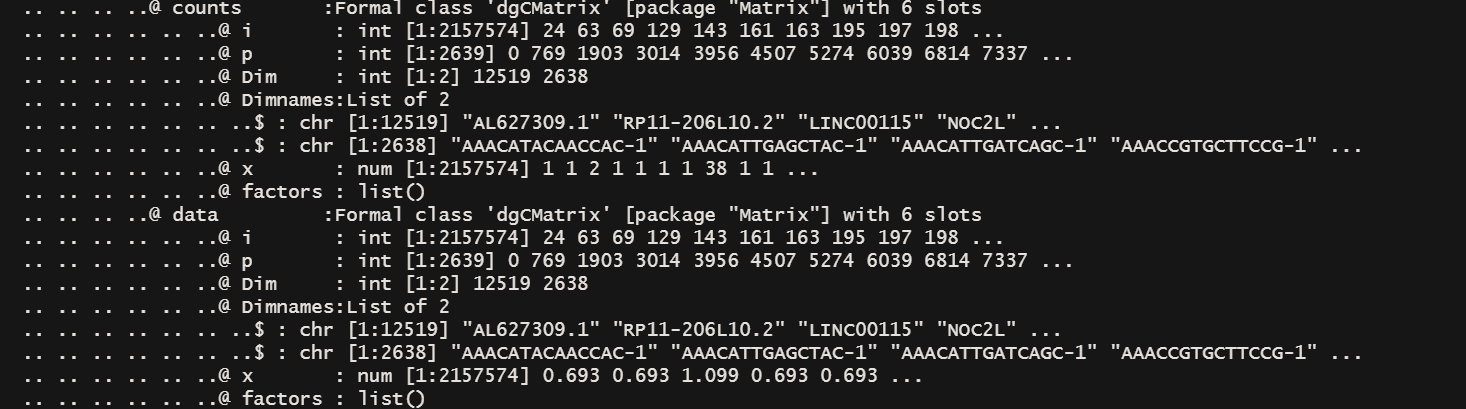
str(pbmc_scT)
# 你去看现在的seurate object数组组织结构发现在asssys slot下多了一个SCT slot，这里面的东西和 RNA slot平级 
# 如果你用LogNormalization 数据会放在 assays$RNA@data@x 下面
# 现在放在了 assays$SCT@data@x 下面

pbmc_logN <- NormalizeData(pbmc, normalization.method = "LogNormalize", scale.factor = 10000)
pbmc_scT <- SCTransform(pbmc, vst.flavor = "v2")

opar <- par(no.readonly=TRUE)
par(mfrow=c(1,2))
hist(pbmc_logN[["RNA"]]@data["MT-ND4",],main = "LogNormalize",xlab = "")
hist(pbmc_scT[["SCT"]]@data["MT-ND4",],main = "SCTransform",xlab = "")
par(opar)

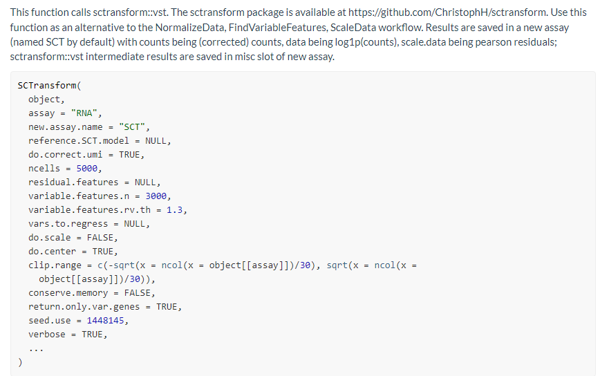
仔细去看看这个函数

• assay
  Name of assay to pull the count data from; default is ‘RNA’

• do.correct.umi
  Place corrected UMI matrix in assay counts slot; default is TRUE
  我读到这里才发现改函数还会对原始的counts数据进行矫正，然后放到assays@SCT$counts@x下面

• ncells
  Number of subsampling cells used to build NB regression; default is 5000

• residual.features
  Genes to calculate residual features for; default is NULL (all genes). If specified, will be set to VariableFeatures of the returned object.

• variable.features.n
  Use this many features as variable features after ranking by residual variance; default is 3000. Only applied if residual.features is not set.

• variable.features.rv.th
  Instead of setting a fixed number of variable features, use this residual variance cutoff; this is only used when variable.features.n is set to NULL; default is 1.3. Only applied if residual.features is not set.

• vars.to.regress
  Variables to regress out in a second non-regularized linear regression. For example, percent.mito. Default is NULL

• do.scale
  Whether to scale residuals to have unit variance; default is FALSE

• do.center
  Whether to center residuals to have mean zero; default is TRUE

• clip.range
  Range to clip the residuals to; default is c(-sqrt(n/30), sqrt(n/30)), where n is the number of cells

• return.only.var.genes
  If set to TRUE the scale.data matrices in output assay are subset to contain only the variable genes; default is TRUE

• seed.use
  Set a random seed. By default, sets the seed to 1448145. Setting NULL will not set a seed.

• verbose
  Whether to print messages and progress bars