ADVERSARIAL EXAMPLE GENERATION

研究推动 ML 模型变得更快、更准、更高效。设计和模型的安全性和鲁棒性经常被忽视，尤其是面对那些想愚弄模型故意对抗时。

本教程将提供您对 ML 模型的安全漏洞的认识，并将深入了解对抗性机器学习这一热门话题。在图像中添加难以察觉的扰动会导致模型性能的显著不同，鉴于这是一个教程，我们将通过图像分类器的示例来探讨这个主题。具体来说，我们将使用第一种也是最流行的攻击方法之一，快速梯度符号攻击（ FGSM ）来欺骗 MNIST 分类器。

Threat Model (攻击模型)

在论文中，有许多类型的对抗攻击，每种攻击都有不同的目标和攻击者的知识假设。然而，总的来说，首要目标是向输入数据添加最小数量的扰动，以导致期望的错误分类。攻击者的知识有几种假设，其中两种是： white-box (白盒)和 black-box （黑盒）；白盒攻击假定攻击者具有对模型的完整知识和访问权限，包括体系结构、输入、输出和权重。黑盒攻击假设攻击者只能访问模型的输入和输出，并且对底层架构或权重一无所知。还有几种类型的目标，包括 misclassification （错误分类）和 source/target misclassification 源/目标错误分类。错误分类的目标意味着对手只希望输出分类错误，而不在乎新的分类是什么。源/目标错误分类意味着对手希望更改最初属于特定源类别的图像，从而将其分类为特定目标类别。

Fast Gradient Sign Attack

FGSM 攻击是白盒攻击，目标是错误分类。

迄今为止最早也是最流行的的对抗攻击是 Fast Gradient Sign Attack, FGSM （Explaining and Harnessing Adversarial Examples），这种攻击非常强大，也很直观。它旨在利用神经网络的学习方式，即梯度来攻击神经网络。这个想法很简单，而不是通过基于反向传播梯度调整权重来最小化损失，而是基于相同的反向传播梯度来调整输入数据以最大化损失。换句话说，攻击使用输入数据的损失梯度，然后调整输入数据以最大化损失。

在这里插入图片描述

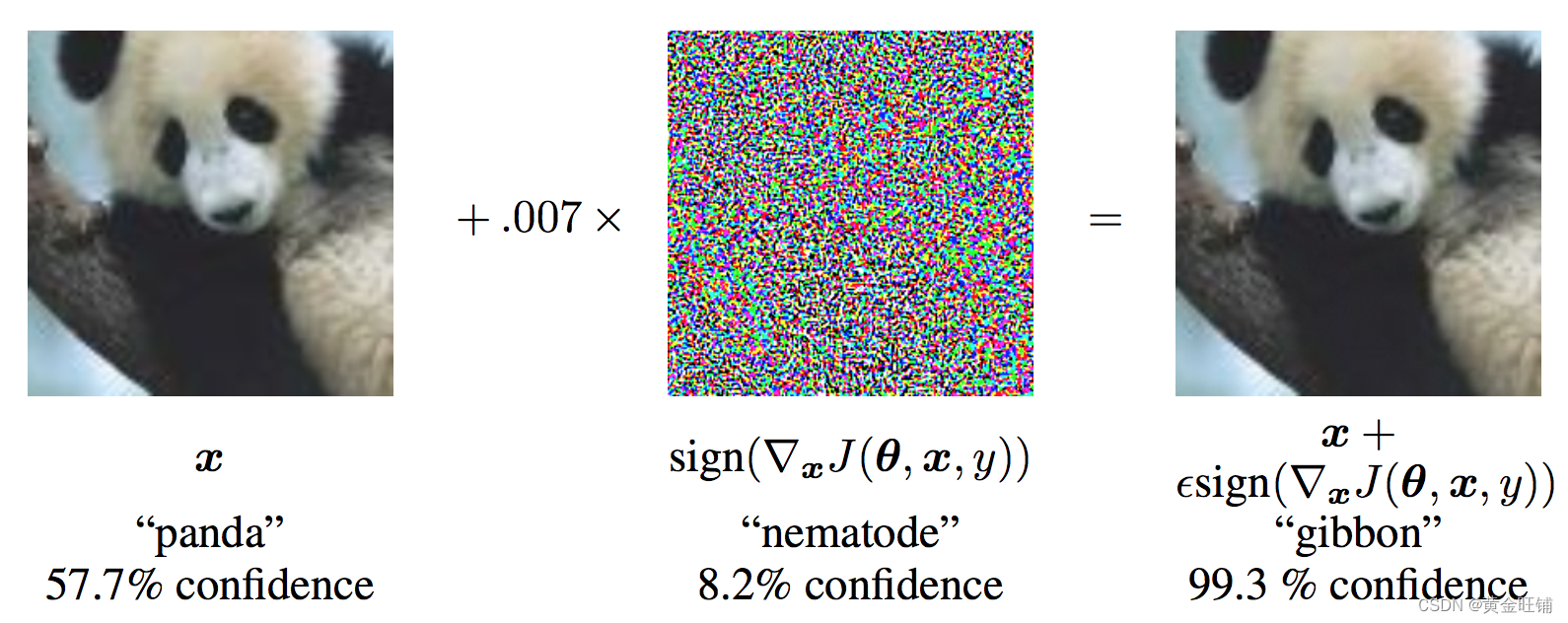
从图中可以看出， $x$ 是被正确分类为 panda 的原始图像， $y$ 是 $x$ 的正确标签， $\theta$ 代表的是模型参数，$ J(\theta, x, y)$ 是训练网络的 loss 。攻击反向传播梯度到输入数据计算 $\nabla_x J(\theta, x, y)$ , 然后利用很小的步长（ $\epsilon$ 或 0.007 ）在某个方向上最大化损失（例如： $sign(\nabla_x J(\theta, x, y))$ ），最后的扰动图像 $x^{'}$ 最后被错误分类为 gibbon, 实际上图像还是 panda 。

import torch
import torch.nn as nn 
import torch.nn.functional as F 
import torch.optim as optim 
from torchvision import datasets, transforms 
import numpy as np 
import matplotlib.pyplot as plt 

from six.moves import urllib 
opener = urllib.request.build_opener() 
opener.addheaders = [('User-agent', 'Mozilla/5.0')] 
urllib.request.install_opener(opener)

Implementation

本节中，我们将讨论教程的输入参数，定义攻击下的模型，以及相关的测试

Inputs

三个输入：

epsilons: epsilon 列表值，保持 0 在列表中非常重要，代表着原始模型的性能。 epsilon 越大代表着攻击越大。
pretrained_model: 预训练模型，训练模型的代码在这里. 也可以直接下载预训练模型. 因为 google drive 无法下载，所以还可以在 CSDN资源下载
use_cuda: 使用 GPU；

Model Under Attack

定义了模型和 DataLoader，初始化模型和加载权重。

class Net(nn.Module):
    def __init__(self):
        super(Net, self).__init__()
        self.conv1 = nn.Conv2d(1, 32, 3, 1)
        self.conv2 = nn.Conv2d(32, 64, 3, 1)
        self.dropout1 = nn.Dropout(0.25)
        self.dropout2 = nn.Dropout(0.5)
        self.fc1 = nn.Linear(9216, 128)
        self.fc2 = nn.Linear(128, 10)

    def forward(self, x):
        x = self.conv1(x)
        x = F.relu(x)
        x = self.conv2(x)
        x = F.relu(x)
        x = F.max_pool2d(x, 2)
        x = self.dropout1(x)
        x = torch.flatten(x, 1)
        x = self.fc1(x)
        x = F.relu(x)
        x = self.dropout2(x)
        x = self.fc2(x)
        output = F.log_softmax(x, dim=1)
        return output


epsilons = [0, .05, .1, .15, .2, .25, .3]
pretrained_model = "lenet_mnist_model.pt"
use_cuda = True

# MNIST Test dataset and dataloader declaration
test_loader = torch.utils.data.DataLoader(
    datasets.MNIST('../../../datasets', train=False, download=True, transform=transforms.Compose([
        transforms.ToTensor(),
    ])),
    batch_size=1, shuffle=True)

print("CUDA Available: ", torch.cuda.is_available())
device = torch.device('cuda' if (use_cuda and torch.cuda.is_available()) else 'cpu')

# init network
model = Net().to(device)

# load the pretrained model 
model.load_state_dict(torch.load(pretrained_model, map_location='cpu'))

# set the model in evaluation mode. In this case this is for the Dropout layers
model.eval()

CUDA Available:  True
Net(
  (conv1): Conv2d(1, 32, kernel_size=(3, 3), stride=(1, 1))
  (conv2): Conv2d(32, 64, kernel_size=(3, 3), stride=(1, 1))
  (dropout1): Dropout(p=0.25, inplace=False)
  (dropout2): Dropout(p=0.5, inplace=False)
  (fc1): Linear(in_features=9216, out_features=128, bias=True)
  (fc2): Linear(in_features=128, out_features=10, bias=True)
)

FGSM Attack （FGSM 攻击）

我们现在定义一个函数创建一个对抗实例，通过对原始输入进行干扰。 fgsm_attack 函数有3个输入，原始输入图像 $x$ ，像素方向扰动量 $\epsilon$ ，梯度损失，（例如 $\nabla_x J(\mathbf{\theta}, \mathbf{x}, y)$ ）

创建干扰图像

$perturbed_image=image+epsilon∗sign(data_grad)=x+ϵ∗sign(∇x J(θ,x,y))$

最后，为了保持原始图像的数据范围，干扰图像被缩放到 [0, 1]

# FGSM attack code
def fgsm_attack(image, epsilon, data_grad):
    # collect the element-wise sign of the data gradient
    sign_data_grad = data_grad.sign()
    
    # create the perturbed image by adjusting each pixel of the input image 
    perturbed_image = image + epsilon * sign_data_grad 
    
    # adding clipping to maintain [0, 1] range 
    perturbed_image = torch.clamp(perturbed_image, 0, 1)
    
    # return the perturbed image 
    return perturbed_image

Testing Function （测试函数）

def test(model, device, test_loader, epsilon):
    # accuracy counter
    correct = 0
    adv_examples = []
    
    # loop over all examples in test set 
    for data, target in test_loader:
        data, target = data.to(device), target.to(device)
        
        # Set requires_grad attribute of tensor. Important for Attack
        data.requires_grad = True
        
        # 
        output = model(data)
        init_pred = output.max(1, keepdim=True)[1]
        
        # if the initial prediction is wrong, don't botter attacking, just move on
        if init_pred.item() != target.item():
            continue 
        
        # calculate the loss
        loss = F.nll_loss(output, target)
        
        # zero all existing grad
        model.zero_grad()

        # calculate gradients of model in backward loss 
        loss.backward()
        
        # collect datagrad
        data_grad = data.grad.data 
        
        # call FGSM attack
        perturbed_data = fgsm_attack(data, epsilon, data_grad)
        
        # reclassify the perturbed image 
        output = model(perturbed_data)
        
        # check for success 
        final_pred = output.max(1, keepdim=True)[1]
        
        # 
        if final_pred.item() == target.item():
            correct += 1
            
            # special case for saving 0 epsilon examples
            if (epsilon == 0) and (len(adv_examples) < 5):
                adv_ex = perturbed_data.squeeze().detach().cpu().numpy()
                adv_examples.append((init_pred.item(), final_pred.item(), adv_ex))
        else:
            # Save some adv examples for visualization later
            if len(adv_examples) < 5:
                adv_ex = perturbed_data.squeeze().detach().cpu().numpy()
                adv_examples.append( (init_pred.item(), final_pred.item(), adv_ex) )

    # Calculate final accuracy for this epsilon
    final_acc = correct/float(len(test_loader))
    print("Epsilon: {}\tTest Accuracy = {} / {} = {}".format(epsilon, correct, 
        len(test_loader), final_acc))

    # Return the accuracy and an adversarial example
    return final_acc, adv_examples

Run Attack (执行攻击)

实现的最后一步是执行攻击，我们针对每个 epsilon 执行全部的 test step，并且保存最终的准确率和一些成功的对抗实例。 $\epsilon=0$ 不执行攻击

accuracies = []
examples = []

# Run test for each epsilon
for eps in epsilons:
    acc, ex = test(model, device, test_loader, eps)
    accuracies.append(acc)
    examples.append(ex)

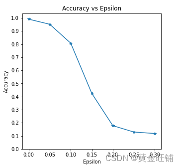
Epsilon: 0	Test Accuracy = 9906 / 10000 = 0.9906
Epsilon: 0.05	Test Accuracy = 9517 / 10000 = 0.9517
Epsilon: 0.1	Test Accuracy = 8070 / 10000 = 0.807
Epsilon: 0.15	Test Accuracy = 4242 / 10000 = 0.4242
Epsilon: 0.2	Test Accuracy = 1780 / 10000 = 0.178
Epsilon: 0.25	Test Accuracy = 1292 / 10000 = 0.1292
Epsilon: 0.3	Test Accuracy = 1180 / 10000 = 0.118

Accuracy vs Epsilon (正确率 VS epsilon)

$\epsilon$ 增大时，我们期望正确率下降，因为大的 $\epsilon$ 我们在方向上有大的变换可以最大化 loss. 他们的变换不是线性的，一开始下降的慢，中间下降的快，最后下降的慢。

plt.figure(figsize=(5, 5))
plt.plot(epsilons, accuracies, "*-")
plt.yticks(np.arange(0, 1.1, step=0.1))
plt.xticks(np.arange(0, .35, step=0.05))
plt.title("Accuracy vs Epsilon")
plt.xlabel("Epsilon")
plt.ylabel("Accuracy")
plt.show()

在这里插入图片描述

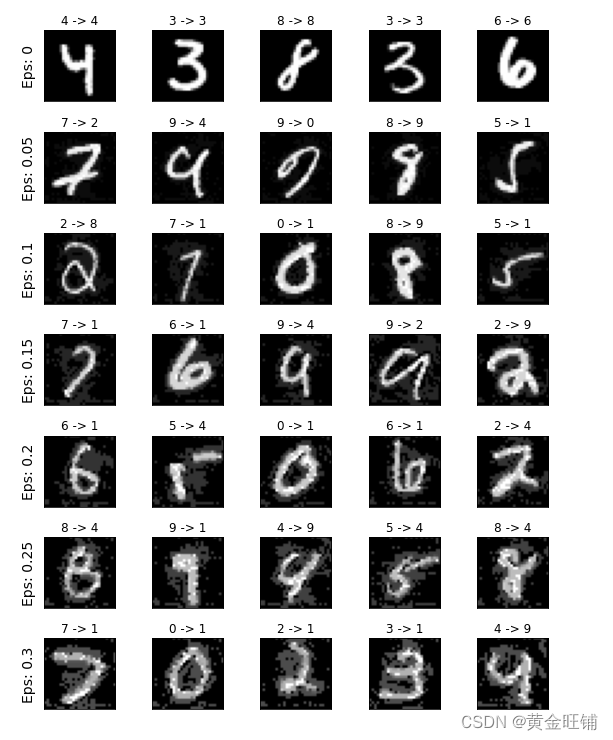
Sample Adversarial Examples (对抗实例)

# Plot several examples of adversarial samples at each epsilon
cnt = 0
plt.figure(figsize=(8,10))
for i in range(len(epsilons)):
    for j in range(len(examples[i])):
        cnt += 1
        plt.subplot(len(epsilons),len(examples[0]),cnt)
        plt.xticks([], [])
        plt.yticks([], [])
        if j == 0:
            plt.ylabel("Eps: {}".format(epsilons[i]), fontsize=14)
        orig,adv,ex = examples[i][j]
        plt.title("{} -> {}".format(orig, adv))
        plt.imshow(ex, cmap="gray")
plt.tight_layout()
plt.show()

在这里插入图片描述

完整代码

import torch
import torch.nn as nn 
import torch.nn.functional as F 
import torch.optim as optim 
from torchvision import datasets, transforms 
import numpy as np 
import matplotlib.pyplot as plt 

from six.moves import urllib 
opener = urllib.request.build_opener() 
opener.addheaders = [('User-agent', 'Mozilla/5.0')] 
urllib.request.install_opener(opener) 

class Net(nn.Module):
    def __init__(self):
        super(Net, self).__init__()
        self.conv1 = nn.Conv2d(1, 32, 3, 1)
        self.conv2 = nn.Conv2d(32, 64, 3, 1)
        self.dropout1 = nn.Dropout(0.25)
        self.dropout2 = nn.Dropout(0.5)
        self.fc1 = nn.Linear(9216, 128)
        self.fc2 = nn.Linear(128, 10)

    def forward(self, x):
        x = self.conv1(x)
        x = F.relu(x)
        x = self.conv2(x)
        x = F.relu(x)
        x = F.max_pool2d(x, 2)
        x = self.dropout1(x)
        x = torch.flatten(x, 1)
        x = self.fc1(x)
        x = F.relu(x)
        x = self.dropout2(x)
        x = self.fc2(x)
        output = F.log_softmax(x, dim=1)
        return output


epsilons = [0, .05, .1, .15, .2, .25, .3]
pretrained_model = "lenet_mnist_model.pt"
use_cuda = True

# MNIST Test dataset and dataloader declaration
test_loader = torch.utils.data.DataLoader(
    datasets.MNIST('../../../datasets', train=False, download=True, transform=transforms.Compose([
        transforms.ToTensor(),
    ])),
    batch_size=1, shuffle=True)

print("CUDA Available: ", torch.cuda.is_available())
device = torch.device('cuda' if (use_cuda and torch.cuda.is_available()) else 'cpu')

# init network
model = Net().to(device)

# load the pretrained model 
model.load_state_dict(torch.load(pretrained_model, map_location='cpu'))

# set the model in evaluation mode. In this case this is for the Dropout layers
model.eval()

# FGSM attack code
def fgsm_attack(image, epsilon, data_grad):
    # collect the element-wise sign of the data gradient
    sign_data_grad = data_grad.sign()
    
    # create the perturbed image by adjusting each pixel of the input image 
    perturbed_image = image + epsilon * sign_data_grad 
    
    # adding clipping to maintain [0, 1] range 
    perturbed_image = torch.clamp(perturbed_image, 0, 1)
    
    # return the perturbed image 
    return perturbed_image


def test(model, device, test_loader, epsilon):
    # accuracy counter
    correct = 0
    adv_examples = []

    # loop over all examples in test set
    for data, target in test_loader:
        data, target = data.to(device), target.to(device)

        # Set requires_grad attribute of tensor. Important for Attack
        data.requires_grad = True

        #
        output = model(data)
        init_pred = output.max(1, keepdim=True)[1]

        # if the initial prediction is wrong, don't botter attacking, just move on
        if init_pred.item() != target.item():
            continue

        # calculate the loss
        loss = F.nll_loss(output, target)

        # zero all existing grad
        model.zero_grad()

        # calculate gradients of model in backward loss
        loss.backward()

        # collect datagrad
        data_grad = data.grad.data

        # call FGSM attack
        perturbed_data = fgsm_attack(data, epsilon, data_grad)

        # reclassify the perturbed image
        output = model(perturbed_data)

        # check for success
        final_pred = output.max(1, keepdim=True)[1]

        #
        if final_pred.item() == target.item():
            correct += 1

            # special case for saving 0 epsilon examples
            if (epsilon == 0) and (len(adv_examples) < 5):
                adv_ex = perturbed_data.squeeze().detach().cpu().numpy()
                adv_examples.append(
                    (init_pred.item(), final_pred.item(), adv_ex))
        else:
            # Save some adv examples for visualization later
            if len(adv_examples) < 5:
                adv_ex = perturbed_data.squeeze().detach().cpu().numpy()
                adv_examples.append(
                    (init_pred.item(), final_pred.item(), adv_ex))

    # Calculate final accuracy for this epsilon
    final_acc = correct/float(len(test_loader))
    print("Epsilon: {}\tTest Accuracy = {} / {} = {}".format(epsilon, correct,
                                                             len(test_loader), final_acc))

    # Return the accuracy and an adversarial example
    return final_acc, adv_examples


accuracies = []
examples = []

# Run test for each epsilon
for eps in epsilons:
    acc, ex = test(model, device, test_loader, eps)
    accuracies.append(acc)
    examples.append(ex)

plt.figure(figsize=(5, 5))
plt.plot(epsilons, accuracies, "*-")
plt.yticks(np.arange(0, 1.1, step=0.1))
plt.xticks(np.arange(0, .35, step=0.05))
plt.title("Accuracy vs Epsilon")
plt.xlabel("Epsilon")
plt.ylabel("Accuracy")
plt.show()


# Plot several examples of adversarial samples at each epsilon
cnt = 0
plt.figure(figsize=(8, 10))
for i in range(len(epsilons)):
    for j in range(len(examples[i])):
        cnt += 1
        plt.subplot(len(epsilons), len(examples[0]), cnt)
        plt.xticks([], [])
        plt.yticks([], [])
        if j == 0:
            plt.ylabel("Eps: {}".format(epsilons[i]), fontsize=14)
        orig, adv, ex = examples[i][j]
        plt.title("{} -> {}".format(orig, adv))
        plt.imshow(ex, cmap="gray")
plt.tight_layout()
plt.show()