摘要

在本周阅读的论文中，作者提出了一种名为MGSFformer的空气质量预测模型。模型通过残差去冗余模块可以有效解耦多粒度数据间的信息重叠；时空注意力模块采用并行建模策略，能够同步挖掘监测站点间的动态空间关联与跨时间步的复杂依赖关系，通过创新性地引入动态权重分配策略实现多粒度预测结果的自适应融合。这一框架突破了传统时空预测模型在冗余信息抑制、多源特征协同与长时预测优化方面的技术瓶颈，通过端到端的深度特征交互机制显著增强了模型对复杂时空演化规律的建模能力，为环境数据的智能分析提供了新的方法支撑。

Abstract

In the paper read this week, the author proposed an air quality prediction model called MGSFformer. The model can effectively decouple the information overlap between multi granularity data by removing redundant modules through residuals; The spatiotemporal attention module adopts a parallel modeling strategy, which can synchronously mine the dynamic spatial correlations and complex dependencies across time steps between monitoring stations. By innovatively introducing a dynamic weight allocation strategy, it achieves adaptive fusion of multi granularity prediction results. This framework breaks through the technical bottlenecks of traditional spatiotemporal prediction models in redundant information suppression, multi-source feature collaboration, and long-term prediction optimization. Through an end-to-end deep feature interaction mechanism, it significantly enhances the model’s ability to model complex spatiotemporal evolution laws, providing new methodological support for intelligent analysis of environmental data.

1. 文献阅读

本周阅读了一篇名为MGSFformer: A Multi-Granularity Spatiotemporal Fusion Transformer for air quality predictiond的论文
论文地址：MGSFformer

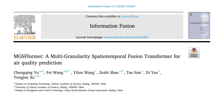
MGSFformer是一种用于空气质量时空预测的模型，通过多粒度数据和时空相关性提升预测精度。论文的创新点分为两部分，第一部分是MGSFformer中三个模块的设计，第二部分是通过统一的端到端框架整合了多粒度和时空特征，从而全面提升预测性能。

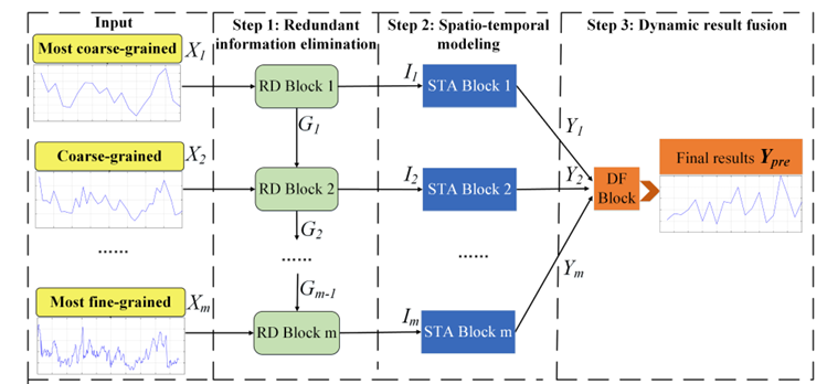
1.1 模型架构

MGSFformer是一种基于Transformer的模型，通过多粒度数据和时空相关性提升预测精度。其核心由三个模块组成：残差去冗余模块、时空注意力模块和动态融合模块，结构如下所示：

RD Block
RD模块主要是为了消除多粒度数据中的冗余信息，其结构如下图所示：

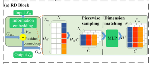
这一模块实现的主要就是输入数据的预处理，其中的information enbedding部分首先将将细粒度数据划分为与粗粒度相同数量的段，转换为3D张量，然后在通过多层感知机将不同粒度的特征映射到统一维度。最后用一个残差链接从细粒度特征中减去粗粒度冗余信息。RD模块通过显式建模冗余对应关系并剔除，防止模型过拟合全局模式。

STA Block
STA模块通过并行的时间注意力和空间注意力捕获序列的时空依赖，交叉注意力整合信息，其结构如下图所示：

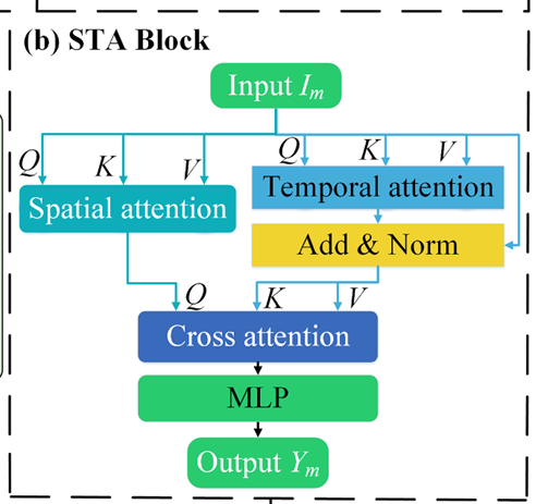
STA模块的主要作用是捕获序列的时空依赖，模块首先分别通过时间注意力机制和空间注意力机制分别计算时间步间的依赖和建模监测站间的空间相关性；然后再通过一个交叉注意力融合时空特征，经MLP层将3D特征转换为预测结果。这以模块通过多级注意力机制显式建模复杂时空依赖，提升了预测精度。

DF Block
DF模块通过注意力机制评估不同粒度预测结果在各时间步的重要性，动态加权求和得到最终预测，其结构如下图所示：

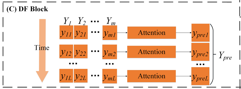
在DF模块中，首先通过注意力机制计算STA模块所得各粒度预测的权重，然后按照计算所得的权重聚合多粒度预测结果，所使用的公式如下所示：

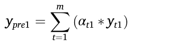
其中的α_t1即是注意力计算所得权重，
以下是对模型工作流程的一个总结：
数据首先进入残差去冗余模块，在这里通过分段采样对齐粗细粒度时间框架，使用MLP识别冗余信息，并通过残差连接从细粒度数据中减去冗余，生成去冗余特征。这些特征流入时空注意力模块，该模块通过并行的空间注意力、时间注意力和交叉注意力机制，分别捕获站点间的空间相关性、时间序列的依赖关系和时空综合特征，生成融合的时空表示。最后，数据进入动态融合模块，该模块利用注意力机制为每个预测时间步计算粗细粒度预测的权重，动态组合这些预测结果，生成最终的空气质量预测输出。

1.2 实验分析

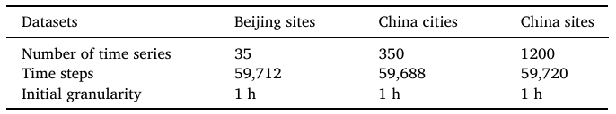
（1）数据集
北京站点:该数据集是来自中国北京35个空气监测站的空气质量数据。数据集的时间范围是从2015年到2021年。数据粒度时间戳包括1天、12小时、6小时、3小时和1小时。
中国城市:此数据集包含从中国350个城市收集的空气质量数据。数据集的时间范围是从2015年到2021.数据粒度时间戳包括1天、12小时、6小时、3小时和1小时。
中国站点:该数据集包含从中国1200个站点收集的空气质量数据。数据集的时间范围是从2015年到2021年。数据粒度时间戳包括1天、12小时、6小时、3小时和1小时。

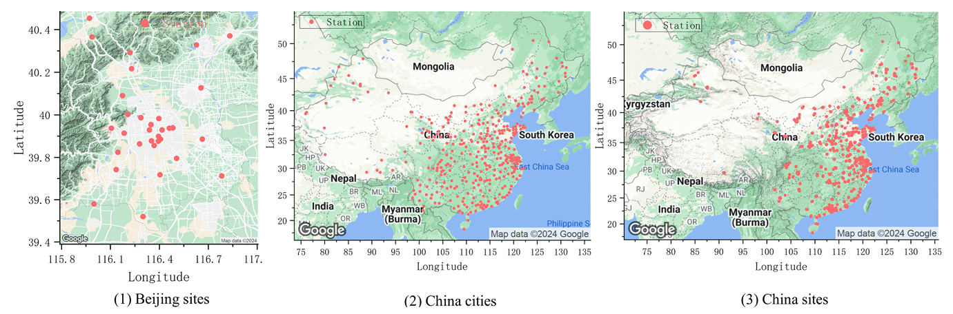
站点分布情况：

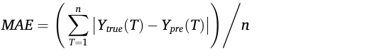
（2）评估标准
MAE:

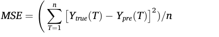
MSE:

CORR:

对比的基线模型有VAR、GRU、LSTNet、TimesNet 、SciNet、MegaCRN、AGCRN、TimeMixer 、PatchFormerDSformer、Airformer。

（3）实验分析
1）性能分析
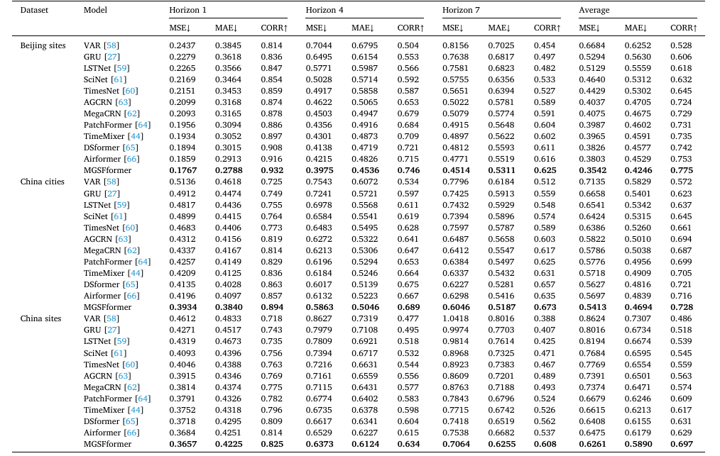
这部分实验是为了比较MGSFformer与基线模型（如VAR、GRU、Airformer）的预测准确性，其结果如下：
不同模型的效率：

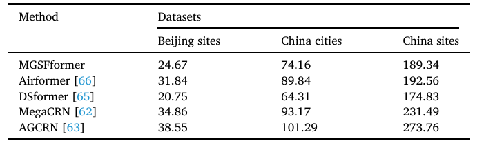
所有模型在AQI数据集上的实验结果：

MGSFformer和四种类型空气污染数据的几个基线的预测性能：
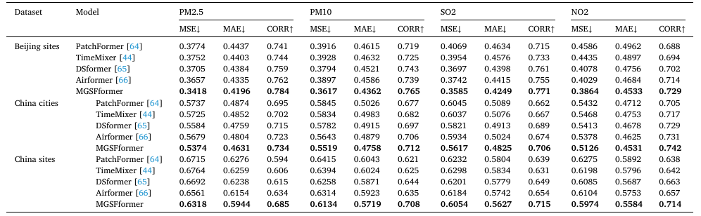与其他经典模型和最先进的模型相比，通过多粒度和时空相关性建模所提出的MGSFformer显著提升了预测精度，取得了最佳结果。
2）组件替换实验
该部分实验主要是为了严重模型中各个组件的重要性，实验通过用其他组件替换论文中的3个模块来进行该部分实验，实验结果如下：

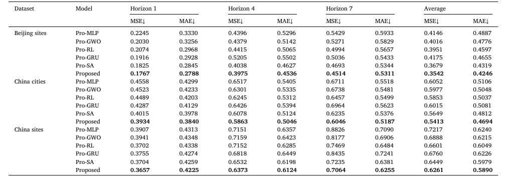
有实验可得无论替换MGSFformer的哪个模块都会导致实验效果下降，各模块设计对模型性能至关重要。
3）消融实验
消融实验的目的是为了确认模型中的各个部分是否是必要的，所得实验结果如下所示：

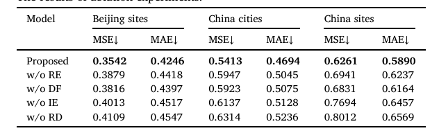
由实验结果可得，MGSFformer中的各个模块都是必要且重要的，RD、残差连接和动态融合是模型成功的关键。
4）多粒度分析
这部分的实验是为了验证多粒度建模的效果，作者通过删减实验中使用到的5个粒度以及只使用单粒度进行实验，实验结果如下：

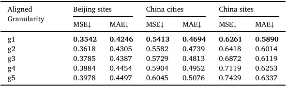
由实验结果可知，多粒度的输入通过提供多样信息，显著提升了预测能力。
5）可视化分析
这部分实验是为了直观地评估模型的性能，作者在时间和空间维度上进行了可视化设计：

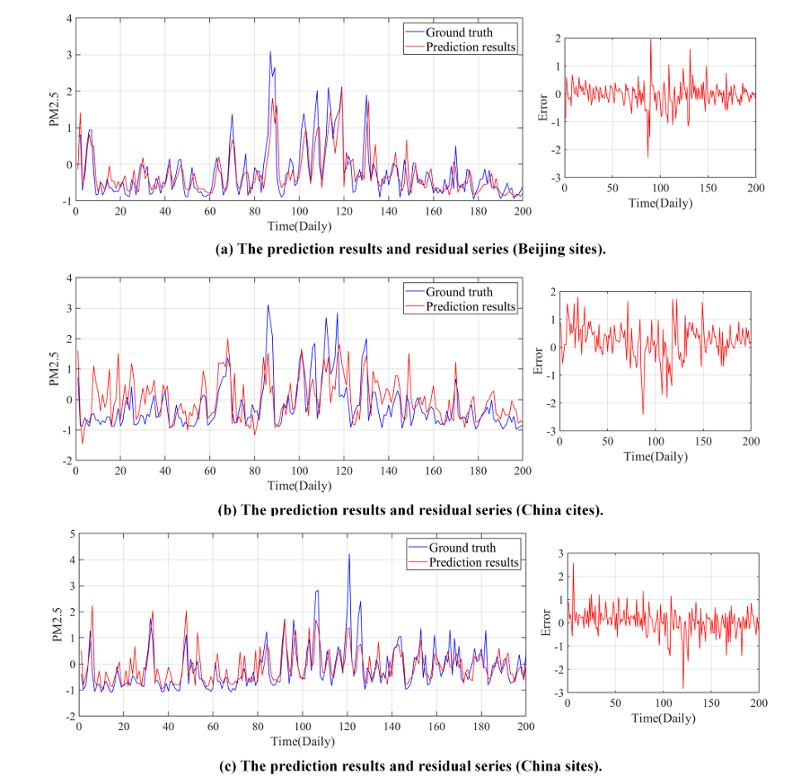
上图显示了所提模型的预测结果和残差级数。可以发现，所提模型接近真实的AQI时间序列。所提出的模型无论是预测突变值还是平滑序列，都取得了令人满意的结果。

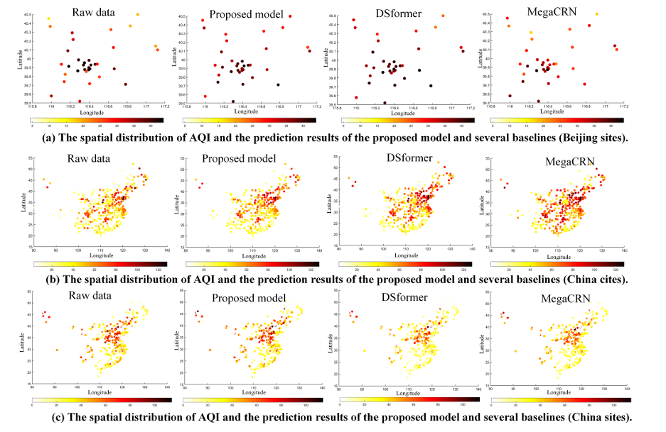
上图显示了几个模型在这三个数据集上的空间预测结果的可视化。根据结果可以发现，AQI呈现局部地区高度集中、其他地区低集中的分布形式。与其他型号相比所提模型的预测结果更接近真实空气质量数据。此外，所提模型可以预测AQI高的区域，为环境治理和个人防护提供参考。

1.3 代码实践

在本周，我通过使用我们实验室的水质数据复现了一个DA-LSTM的模型，对PH值进行了预测，实验结果还算不错，在数据预处理阶段进行了简单的数据清洗将缺失值去除了，实验按照7：3的比例把实验用到的3万条左右的数据划分为训练集和验证集，实验代码如下所示：

import pandas as pd
import numpy as np
from sklearn.preprocessing import MinMaxScaler
import torch
import torch.nn as nn
import torch.optim as optim
import matplotlib.pyplot as plt
import seaborn as sns
import warnings

warnings.filterwarnings('ignore')


# 加载和预处理 CSV 数据集
def load_and_preprocess_data(file_path):
    # 尝试使用不同编码读取 CSV 文件
    encodings = ['gb18030', 'gbk', 'utf-8']
    df = None
    for encoding in encodings:
        try:
            df = pd.read_csv(file_path, encoding=encoding)
            print(f"成功使用 {encoding} 编码读取 CSV 文件")
            break
        except UnicodeDecodeError:
            continue

    if df is None:
        raise ValueError("无法使用以下编码读取 CSV 文件：gb18030, gbk, utf-8")

    # 选择用于预测的特征，包括时间列
    features = ['时间', '水温℃', '溶解氧mg/L', '电导率μs/cm', '浊度NTU',
                '高锰酸盐指数mg/L', '氨氮mg/L', '总磷mg/L', '总氮mg/L', 'pH值无量纲']

    # 检查 CSV 是否包含所有必需列
    missing_cols = [col for col in features if col not in df.columns]
    if missing_cols:
        raise ValueError(f"CSV 文件缺少以下列：{missing_cols}")

    # 数据清洗：替换空字符串或无效值（如 'N/A'）为 NaN
    df = df.replace(['', 'N/A', 'null', 'NaN'], np.nan)

    # 数据清洗：移除任何包含 NaN 的行
    initial_rows = len(df)
    df = df.dropna()
    cleaned_rows = len(df)
    if cleaned_rows < initial_rows:
        print(f"数据清洗：移除了 {initial_rows - cleaned_rows} 行包含缺失值的记录")

    # 验证清洗后数据集非空
    if cleaned_rows == 0:
        raise ValueError("数据清洗后数据集为空，请检查 CSV 文件内容")

    # 处理时间列
    if '时间' in df.columns:
        # 尝试将时间列转换为 datetime，错误值设为 NaT
        df['时间'] = pd.to_datetime(df['时间'], errors='coerce')
        if df['时间'].isna().all():
            print("警告：时间列所有值无效，将不按时间排序")
        else:
            # 按时间排序，移除时间无效的行
            df = df.dropna(subset=['时间']).sort_values('时间').reset_index(drop=True)
    else:
        print("警告：未找到时间列，将不按时间排序")

    # 提取特征（不包括时间列）
    feature_cols = [col for col in features if col != '时间']
    df_features = df[feature_cols]

    # 检查并记录非数值数据
    for col in feature_cols:
        non_numeric = df_features[col][pd.to_numeric(df_features[col], errors='coerce').isna()]
        if not non_numeric.empty:
            print(f"警告：列 {col} 包含非数值数据：{non_numeric.unique()}")

    # 将特征转换为数值类型，错误值转为 NaN
    for col in feature_cols:
        df_features[col] = pd.to_numeric(df_features[col], errors='coerce')

    # 处理剩余的缺失值：使用线性插值
    df_features = df_features.interpolate(method='linear', limit_direction='both')

    # 检查插值后是否仍有缺失值
    if df_features.isna().any().any():
        print("警告：插值后仍存在缺失值，将删除包含 NaN 的行")
        df_features = df_features.dropna()

    # 移除异常值（基于 IQR 方法）
    for col in feature_cols:
        Q1 = df_features[col].quantile(0.25)
        Q3 = df_features[col].quantile(0.75)
        IQR = Q3 - Q1
        lower_bound = Q1 - 1.5 * IQR
        upper_bound = Q3 + 1.5 * IQR
        df_features[col] = df_features[col].clip(lower=lower_bound, upper=upper_bound)

    # 检查特征与 pH 的相关性并绘制热图
    corr = df_features.corr()
    print("\n特征与 pH 的相关性：\n", corr['pH值无量纲'].abs().sort_values(ascending=False))
    plt.figure(figsize=(10, 8))
    sns.heatmap(corr, annot=True, cmap='coolwarm', fmt='.2f')
    plt.title('特征相关性热图')
    plt.savefig('correlation_heatmap.png')
    plt.close()

    # 将处理后的特征放回原始 DataFrame
    df[feature_cols] = df_features

    return df[feature_cols]


# 为 LSTM 创建时间序列（带滑动窗口）
def create_sequences(data, seq_length, target_col_idx, step_size=1):
    X, y = [], []
    # 使用滑动窗口生成更多序列
    for i in range(0, len(data) - seq_length, step_size):
        X.append(data[i:i + seq_length])
        y.append(data[i + seq_length, target_col_idx])
    return np.array(X), np.array(y)


# 定义 PyTorch 中的 LSTM 模型
class LSTMModel(nn.Module):
    def __init__(self, input_size, hidden_size1=64, hidden_size2=32, dropout=0.2):
        super(LSTMModel, self).__init__()
        # 第一个 LSTM 层
        self.lstm1 = nn.LSTM(input_size, hidden_size1, batch_first=True)
        # 第一个 dropout 层
        self.dropout1 = nn.Dropout(dropout)
        # 第二个 LSTM 层
        self.lstm2 = nn.LSTM(hidden_size1, hidden_size2, batch_first=True)
        # 第二个 dropout 层
        self.dropout2 = nn.Dropout(dropout)
        # 第一个全连接层
        self.fc1 = nn.Linear(hidden_size2, 16)
        # ReLU 激活函数
        self.relu = nn.ReLU()
        # 输出层
        self.fc2 = nn.Linear(16, 1)

    def forward(self, x):
        # 前向传播
        out, _ = self.lstm1(x)
        out = self.dropout1(out)
        out, _ = self.lstm2(out)
        out = self.dropout2(out)
        # 取最后一个时间步的输出
        out = self.fc1(out[:, -1, :])
        out = self.relu(out)
        out = self.fc2(out)
        return out


# 将数据转换为 PyTorch 张量
def prepare_tensors(X, y, device):
    # 转换为浮点型张量并移动到指定设备
    X_tensor = torch.tensor(X, dtype=torch.float32).to(device)
    y_tensor = torch.tensor(y, dtype=torch.float32).to(device)
    return X_tensor, y_tensor


# 训练模型
def train_model(model, X_train, y_train, X_val, y_val, epochs, batch_size, device):
    # 定义损失函数和优化器
    criterion = nn.MSELoss()
    optimizer = optim.Adam(model.parameters(), lr=0.001)

    # 创建训练数据加载器
    train_dataset = torch.utils.data.TensorDataset(X_train, y_train)
    train_loader = torch.utils.data.DataLoader(train_dataset, batch_size=batch_size, shuffle=True)

    train_losses = []
    val_losses = []

    # 训练循环
    for epoch in range(epochs):
        model.train()
        epoch_train_loss = 0
        for X_batch, y_batch in train_loader:
            # 清零梯度
            optimizer.zero_grad()
            # 前向传播
            outputs = model(X_batch)
            # 计算损失
            loss = criterion(outputs.squeeze(), y_batch)
            # 反向传播
            loss.backward()
            # 更新参数
            optimizer.step()
            epoch_train_loss += loss.item() * X_batch.size(0)

        # 计算平均训练损失
        epoch_train_loss /= len(X_train)
        train_losses.append(epoch_train_loss)

        # 计算验证损失
        model.eval()
        with torch.no_grad():
            val_outputs = model(X_val)
            val_loss = criterion(val_outputs.squeeze(), y_val).item()
        val_losses.append(val_loss)

        # 每 10 个 epoch 打印一次损失
        if (epoch + 1) % 10 == 0:
            print(f"Epoch [{epoch + 1}/{epochs}], 训练损失: {epoch_train_loss:.6f}, 验证损失: {val_loss:.6f}")

    return train_losses, val_losses


# 绘制结果图
def plot_results(train_losses, val_losses, predictions, actual):
    # 验证输入数据
    if len(predictions) == 0 or len(actual) == 0:
        raise ValueError("预测值或实际值为空，无法绘图")

    # 绘制训练和验证损失
    plt.figure(figsize=(10, 5))
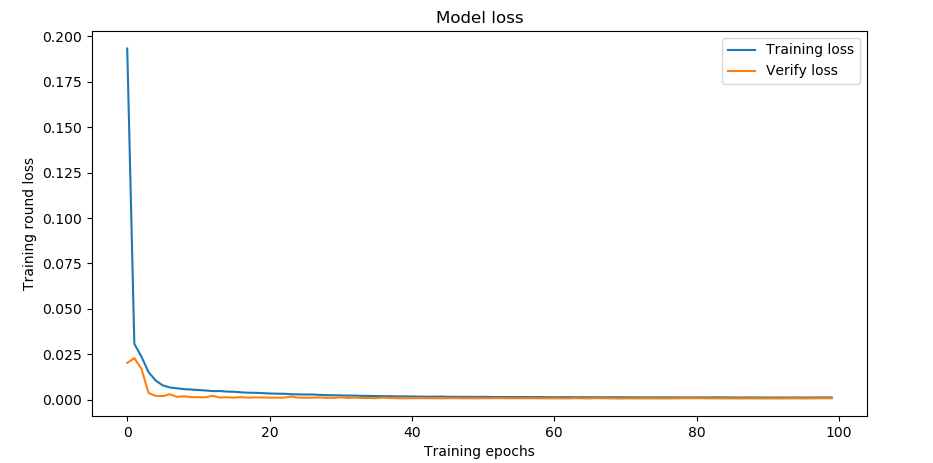
    plt.plot(train_losses, label='训练损失')
    plt.plot(val_losses, label='验证损失')
    plt.title('模型损失')
    plt.xlabel('训练轮次')
    plt.ylabel('损失')
    plt.legend()
    plt.savefig('training_history.png')
    plt.close()

    # 绘制预测值与实际值对比
    plt.figure(figsize=(12, 6))
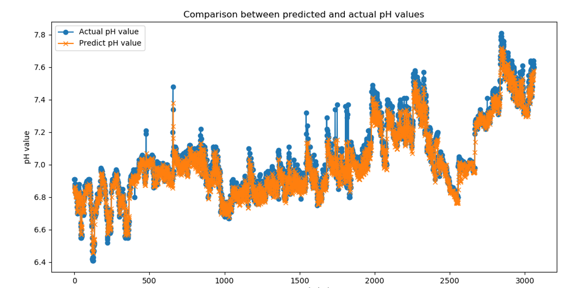
    plt.plot(actual, label='实际 pH 值', marker='o')
    plt.plot(predictions, label='预测 pH 值', marker='x')
    plt.title('预测值与实际 pH 值对比')
    plt.xlabel('测试样本索引')
    plt.ylabel('pH 值')
    plt.legend()
    plt.savefig('predictions_vs_actual.png')
    plt.close()

    # 绘制预测误差分布
    errors = predictions - actual
    plt.figure(figsize=(10, 5))
    plt.hist(errors, bins=30, edgecolor='black')
    plt.title('预测误差分布')
    plt.xlabel('预测误差 (预测值 - 实际值)')
    plt.ylabel('频率')
    plt.savefig('error_distribution.png')
    plt.close()


# 主函数：运行预测流程
def train_and_predict(file_path, seq_length=10, epochs=100,batch_size=320, step_size=1):
    # 设置设备（GPU 或 CPU）
    device = torch.device('cuda' if torch.cuda.is_available() else 'cpu')
    print(f"使用设备: {device}")

    # 加载和预处理数据
    df = load_and_preprocess_data(file_path)

    # 验证数据集大小
    if len(df) < seq_length:
        raise ValueError(f"数据集行数 ({len(df)}) 小于序列长度 ({seq_length})，无法生成序列")

    # 分割训练、验证和测试集（70-10-20）
    train_size = int(0.7 * len(df))
    val_size = int(0.1 * len(df))
    train_df = df[:train_size]
    val_df = df[train_size:train_size + val_size]
    test_df = df[train_size + val_size:]

    # 验证分割后数据集非空
    if len(test_df) == 0:
        raise ValueError("测试集为空，请检查数据分割或数据集大小")

    # 特征缩放（仅基于训练数据拟合 scaler）
    scaler = MinMaxScaler()
    train_scaled = scaler.fit_transform(train_df)
    val_scaled = scaler.transform(val_df)
    test_scaled = scaler.transform(test_df)

    # pH 值是最后一列
    target_col_idx = -1

    # 创建序列（使用滑动窗口）
    X_train, y_train = create_sequences(train_scaled, seq_length, target_col_idx, step_size)
    X_val, y_val = create_sequences(val_scaled, seq_length, target_col_idx, step_size)
    X_test, y_test = create_sequences(test_scaled, seq_length, target_col_idx, step_size)

    # 验证序列非空
    if X_test.shape[0] == 0:
        raise ValueError("测试序列为空，请检查测试集大小或序列长度")

    # 转换为张量
    X_train_tensor, y_train_tensor = prepare_tensors(X_train, y_train, device)
    X_val_tensor, y_val_tensor = prepare_tensors(X_val, y_val, device)
    X_test_tensor, y_test_tensor = prepare_tensors(X_test, y_test, device)

    # 初始化模型并移动到设备
    model = LSTMModel(input_size=X_train.shape[2]).to(device)

    # 训练模型
    train_losses, val_losses = train_model(model, X_train_tensor, y_train_tensor,
                                           X_val_tensor, y_val_tensor, epochs, batch_size, device)

    # 在测试集上评估
    model.eval()
    with torch.no_grad():
        predictions = model(X_test_tensor).cpu().numpy().flatten()  # 确保 1D 数组
        test_mae = np.mean(np.abs(predictions - y_test))
        print(f"\n测试集 MAE（缩放后）: {test_mae:.4f}")

    # 反向转换预测值
    dummy = np.zeros((len(predictions), train_scaled.shape[1]))
    dummy[:, -1] = predictions
    predictions_transformed = scaler.inverse_transform(dummy)[:, -1]

    # 反向转换实际值
    dummy[:, -1] = y_test
    actual_transformed = scaler.inverse_transform(dummy)[:, -1]

    # 打印预测和实际值的形状
    print(f"predictions_transformed shape: {predictions_transformed.shape}, type: {type(predictions_transformed)}")
    print(f"actual_transformed shape: {actual_transformed.shape}, type: {type(actual_transformed)}")

    # 打印样本预测结果
    print("\n样本预测值与实际 pH 值对比：")
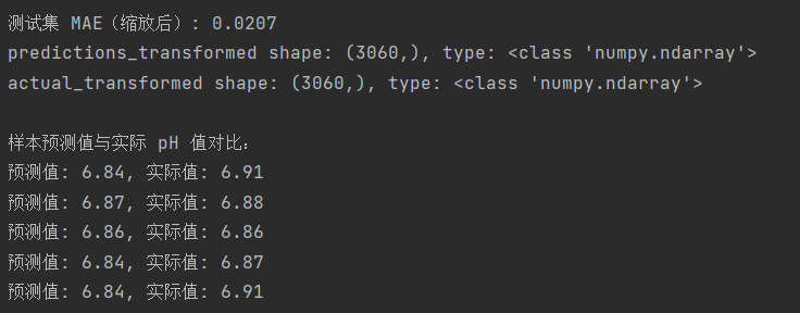
    for i in range(min(5, len(predictions_transformed))):
        print(f"预测值: {predictions_transformed[i]:.2f}, 实际值: {actual_transformed[i]:.2f}")

    # 绘制结果
    plot_results(train_losses, val_losses, predictions_transformed, actual_transformed)

    return model, predictions_transformed, actual_transformed


# 示例用法
if __name__ == "__main__":
    file_path = "1.csv"  # 替换为实际 CSV 文件路径
    model, predictions_transformed, actual_transformed = train_and_predict(file_path)

实验结果如下：
实验所得MAE和真实值与预测值的对比：

训练结果的可视化：

总结

通过本周的学习，我对多粒度数据的输入的优势有了一定的了解，明白了数据预处理对于实验的重要性，本周因为有其他事情需要完成的缘故没有对论文的实验进行复现，在下周的学习中，我会对论文中使用的模型以及实验进行复现。