---

一、理论分析

1. Transformers概述

Transformers由6个encoder和6个decoder组成：

工作流程：

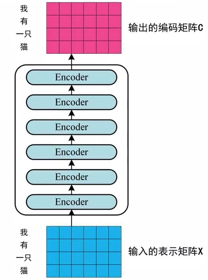
1. 获取输入句子的每一个单词的表示向量$X$，由单词的embedding和位置编码相加得到：
   

2. 将嵌入矩阵$X\in {\mathbb{R}}^{n\times d}$输入到Encoder中，经过6个encoder block后得到句子所有单词的编码信息矩阵$C$，其中$n$是句中单词数量，$d$是单词维度（论文中为$d=512$）
   每一个encoderblock的输出矩阵与输入矩阵形状相同

   

（细节：这里会按照词根来划分token，比如doing会被分成do和ing来编码）

3. 将Encoder输出的编码矩阵$C$传递到Decoder中，Decoder依次会根据当前翻译过的单词$1,2,...,i$来翻译下一个单词$i+1$

   • 实际使用中，翻译到第$i+1$个单词时需要通过Mask来遮盖住$i+1$之后的单词：

   

   • Decoder接收了$C$然后输出一个翻译开始符<Begin>，预测第一个单词$i$
   • 然后输入<Begin> i，预测单词have，以此类推
   • 这是Transformer使用的大致流程

---

2. Transformer的输入部分具体是如何构成？

Transformer 中单词的输入表示 x由单词 Embedding 和位置 Embedding 相加得到。

2.1 单词 Embedding

• 单词的 Embedding 有很多种方式可以获取,
• 例如可以采用 Word2Vec、Glove 等算法预训练得到，也可以在 Transformer 中训练得到。

2.2 位置 Embedding

• Transformer 中除了单词的 Embedding，还需要使用位置 Embedding 表示单词出现在句子中的位置。
• 因为 Transformer 不采用 RNN 的结构，而是使用全局信息，不能利用单词的顺序信息，而这部分信息对于 NLP 来说非常重要。
• 所以 Transformer 中使用位置 Embedding 保存单词在序列中的相对或绝对位置。
• 位置 Embedding用 PE表示，PE的维度与单词 Embedding 是一样的。
• PE 可以通过训练得到，也可以使用某种公式计算得到。在Transformer 中采用了后者，计算公式如下：

$$\begin{gathered} PE(pos,2i)=\sin (pos/10000^{2i/d}) \\ PE(pos,2i+1)=\cos (pos/10000^{2i/d}) \end{gathered}$$

• pos 表示单词在句子中的位置，d表示 PE的维度(与词 Embedding 一样)
• 2i 表示偶数的维度，2i+1表示奇数维度 (即 2i < d, 2i + 1 < d)。

使用这种公式计算PE的好处：

• 使 PE 能够适应比训练集里面所有句子更长的句子，假设训练集里面最长的句子是有 20 个单词，突然来了一个长度为 21 的句子，则使用公式计算的方法可以快速计算出第 21 位的 Embedding。
• 可以让模型容易地计算出相对位置，对于固定长度的间距k，PE(poS+k)可以用 PE(poS)计算得到。因为：

Sin(A+B)=Sin(A)Cos(B)+Cos(A)Sin(B),
Cos(A+B)=Cos(A)Cos(B)-Sin(A)Sin(B)

• 将单词的词 Embedding 和位置 Embedding相加，就可以得到单词的表示向量x，x就是 Transformer 的输入。

---

3 自注意力原理

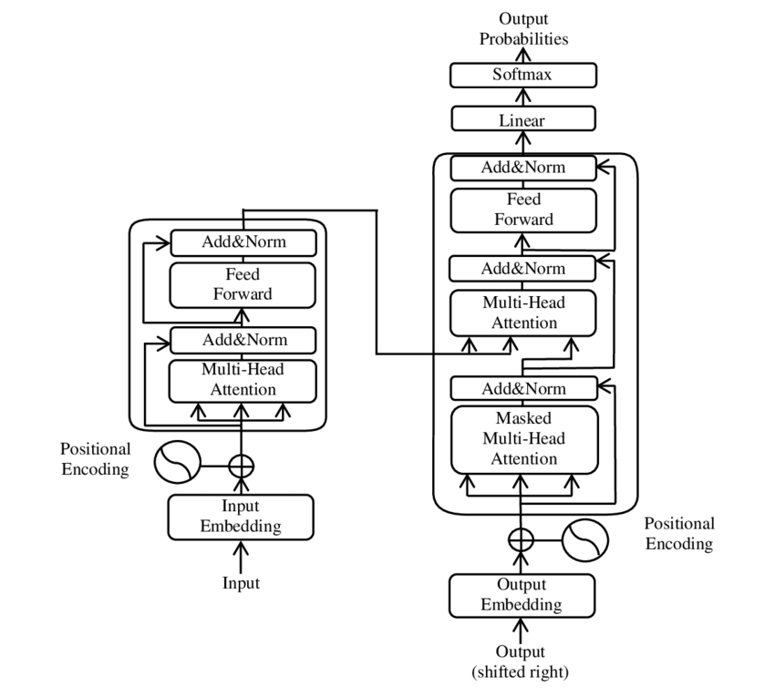
• 红色圈忠的部分是多头注意力，是由多个自注意力组成，可以看到：

  • Encoder包含一个多头注意力
  • Decoder包含两个多头注意力（其中一个用到Mask）

• 多头注意力上方还包括一个AddNorm层，就是残差连接加层正则化（LayerNorm）

3.1 自注意力结构

• 输入：$Q,K,V$
• 实际操作忠，自注意力接收的是输入（单词的表示向量组成的矩阵$X$）或者上一个Encoder block的输出
• $Q,K,V$正是通过自注意力的输入进行线性变换得到

3.2 QKV的计算

自注意力的输入用矩阵$X$表示，则可以使用线性变换矩阵$W_Q,W_K,W_V$计算得到$Q,K,V$，计算如下图所示，注意$X,Q,K,V$的每一行都表示一个单词：

3.3 自注意力的输出

得到矩阵$Q,K,V$之后就可以计算出自注意力的输出了：

$$Att(Q,K,V)=\mathrm{softmax}\left(\frac{Q{K}^{\top }}{\sqrt{d}}\right)V$$

其中$d_k$是$Q,K$的列数，即向量维度，论文中$d=512$

• 公式中计算矩阵$Q$和$K$每一行向量的内积，为了防止内积过大，因此除以$d_k$的平方根
• $Q$乘以$K$的转置后，得到的矩阵行列数都为$n$，$n$为句子单词数，这个矩阵可以表示单词之间的attention强度
• 下图为$Q{K}^{\top }$，1234表示句子中的单词：

• 得到$Q{K}^{\top }$之后，使用softmax计算每一个单词对于其他单词的attention系数
• 公式中的softmax是对矩阵的每一行进行softmax，即每一行的和都变为1

• 得到softmax矩阵后可以和$V$相乘，得到最终输出$Z$

• 上图中Softmax矩阵的第一行表示单词1和其他所有单词的attention系数
• 最终单词1和输出$Z_1$等于所有单词$i$的值$V_i$根据attention系数的比例加在一起得到，如下图所示：

3.4 多头注意力

1. 首先将输入$X$分别传递到$h$个不同的自注意力中，计算得到$h$个输出矩阵$Z$，论文中$h=8$，即得到8个输出矩阵$Z$
   

2. 得到$Z_1$到$Z_8$之后，多头就是直接拼接，然后传入到Linear层，得到多头注意力最终输出$\mathbf{Z}$，这里$\mathbf{Z}$其实和那个是一个形状的。

---

4 Encoder结构

编码器由多头注意力，残差连接+正则（ADD&NORM），前馈和**残差连接+正则（ADD&NORM）**组成

4.1 AddNorm

$$\begin{gathered} LayerNorm(X+MultiHeadAtt(X)) \\ LayerNorm(X+FeedForward(X)) \end{gathered}$$

4.2 前馈

两层的全连接层，第一层激活用ReLU，第二层不用激活：

$$\max (0,X{W}_1+b_1)W_2+b_2$$

4.3 组成Encoder

Encoder block接收输入矩阵$X\in {\mathbb{R}}^{n\times d}$，输出$O\in {\mathbb{R}}^{n\times d}$，通过多个Encoder block叠加得到Encoder

• 第一个Encoder的输入是句子单词的表示向量矩阵
• 后续Encoder的输入是前一个Encoder的输出
• 最后一个Encoder的输出就是编码信息矩阵$C$，

---

二、代码实现细节

video

import torch
from torch import nn
import torch.nn.functional as F
import numpy as np
import pandas as pd
import matplotlib.pyplot as plt
import matplotlib as mpl
from IPython.display import Image
# default: 100
mpl.rcParams['figure.dpi'] = 150

torch.manual_seed(42)

• pytorch transformer (seq modeling) => transformers (hf, focus on language models) => LLM
• pytorch
  • nn.TransformerEncoderLayer => nn.TransformerEncoder
    • TransformerEncoder is a stack of N encoder layers.
    • BERT
  • nn.TransformerDecoderLayer => nn.TransformerDecoder
    • TransformerDecoder is a stack of N decoder layers.
    • GPT
• decoder 与 encoder 相比，有两个特殊的 attention sublayers
  • masked multi-head (self) attention
  • encoder-decoder (cross) attention
    • (k, v) from encoder （memory, last encoder layer）
    • q：decoder input
    • multihead_attn(x, mem, mem) from TransformerDecoderLayer
  • 两者权值不共享

(masked) multi-head attention

https://pytorch.org/docs/stable/generated/torch.nn.functional.scaled_dot_product_attention.html

• Encoder Self-Attention:
  • No Masking:
    • Since attn_bias is zero, the attention weights depend solely on the scaled dot product:
      $${\text{Scores}}_{\text{encoder}}=\frac{Q{K}^{\top }}{\sqrt{d_k}}$$
      $${\text{Attention}}_{\text{encoder}}=\text{softmax}({\text{Scores}}_{\text{encoder}})$$
    • Each token attends to all tokens, including future ones.
• Decoder Masked Self-Attention:
  • Causal Masking:
    • The mask M is defined as:
      $$M_{i,j}=\{\begin{array}{ll}0& \text{if }j\le i\\ -\infty & \text{if }j>i\end{array}$$
    • The attention scores become:
      $${\text{Scores}}_{\text{decoder}}=\frac{Q{K}^{\top }}{\sqrt{d_k}}+M$$
    • Applying softmax:
      $${\text{Attention}}_{\text{decoder}}=\text{softmax}({\text{Scores}}_{\text{decoder}})$$
      • The -inf in M ensures that positions where ( j > i ) (future positions) have zero attention weight.

encoder layer & encoder

• input: $\mathbf{X}\in {\mathbb{R}}^{T\times B\times d_{\text{model}}}$
• 1. multihead selfattn
  • 线性变换（linear projection, 矩阵乘法）生成 Q、K、V矩阵
  • $X_{\text{flat}}=\mathbf{X}.\text{reshape}(T\times B,d_{model})$
  • $\mathbf{QKV}=\mathbf{X}{\mathbf{W}}_{in}^T+{\mathbf{b}}_{in}$（encoder_layer.self_attn.in_proj_weight, encoder_layer.self_attn.in_proj_bias）
    • ${\mathbf{W}}_{in}\in {\mathbb{R}}^{3d_{\text{model}}\times d_{\text{model}}}$，${\mathbf{b}}_{in}\in {\mathbb{R}}^{3d_{\text{model}}}$
    • $\mathbf{QKV}\in {\mathbb{R}}^{T\times B,3d_{model}}$
  • 拆分 $\mathbf{Q},\mathbf{K},\mathbf{V}$
    • $\mathbf{Q},\mathbf{K},\mathbf{V}=\text{split}(\mathbf{QKV},d_{model})$（按列进行拆分）
    • $\mathbf{Q},\mathbf{K},\mathbf{V}\in {\mathbb{R}}^{T\times B,d_{\text{model}}}$
  • 调整形状以适应多头注意力
    • $d_k=\frac{d_{\text{model}}}{h}$
    • reshape_for_heads
      $$\begin{array}{rl}{\mathbf{Q}}_{\text{heads}}& =\mathbf{Q}.\text{reshape}(T,B,h,d_k).\text{permute}(1,2,0,3).\text{reshape}(B\times h,T,d_k)\\ {\mathbf{K}}_{\text{heads}}& =\mathbf{K}.\text{reshape}(T,B,h,d_k).\text{permute}(1,2,0,3).\text{reshape}(B\times h,T,d_k)\\ {\mathbf{V}}_{\text{heads}}& =\mathbf{V}.\text{reshape}(T,B,h,d_k).\text{permute}(1,2,0,3).\text{reshape}(B\times h,T,d_k)\end{array}$$
  • 计算注意力分数：$\text{Scores}=\frac{{\mathbf{Q}}_{\text{heads}}{\mathbf{K}}_{\text{heads}}^{\top }}{\sqrt{d_k}}$
    • ${\mathbf{Q}}_{\text{heads}}\in {\mathbb{R}}^{(B\times h)\times T\times d_k}$，${\mathbf{K}}_{\text{heads}}^{\top }\in {\mathbb{R}}^{(B\times h)\times d_k\times T}$，因此 $\text{Scores}\in {\mathbb{R}}^{(B\times h)\times T\times T}$。
  • 计算注意力权重：$\text{AttentionWeights}=\text{softmax}(\text{Scores})$
  • 计算注意力输出：$\text{AttentionOutput}=\text{AttentionWeights}\times {\mathbf{V}}_{\text{heads}}$
    • ${\mathbf{V}}_{\text{heads}}\in {\mathbb{R}}^{(B\times h)\times T\times d_k}$，因此 $\text{AttentionOutput}\in {\mathbb{R}}^{(B\times h)\times T\times d_k}$。
  • 合并多头输出：$\text{AttentionOutput}=\text{AttentionOutput}.\text{reshape}(B,h,T,d_k).\text{permute}(2,0,1,3).\text{reshape}(T,B,d_{\text{model}})$
  • 输出线性变换：$\text{AttnOutputProjected}=\text{AttentionOutput}{\mathbf{W}}_{\text{out}}^{\top }+{\mathbf{b}}_{\text{out}}$
    • ${\mathbf{W}}_{\text{out}}\in {\mathbb{R}}^{d{}_{\text{model}}\times d_{\text{model}}}$，${\mathbf{b}}_{\text{out}}\in {\mathbb{R}}^{d_{\text{model}}}$，对应代码中的out_proj_weight和out_proj_bias。
• 2. 残差连接和层归一化（第一层）
  • 残差连接：$\text{Residual1}=\mathbf{X}+\text{AttnOutputProjected}$
  • 层归一化：$\text{Normalized1}=\text{LayerNorm}(\text{Residual1},{\gamma }_{\text{norm1}},{\beta }_{\text{norm1}})$
    • ${\gamma }_{\text{norm1}},{\beta }_{\text{norm1}}\in {\mathbb{R}}^{d_{\text{model}}}$，对应代码中的norm1.weight 和 norm1.bias。
• 3. 前馈神经网络 (ffn)
  • 第一层线性变换和激活函数：$\text{FFNOutput1}=\text{ReLU}(\text{Normalized1}{\mathbf{W}}_1^{\top }+{\mathbf{b}}_1)$
    • 其中，${\mathbf{W}}_1\in {\mathbb{R}}^{d_{\text{ff}}\times d_{\text{model}}}$，${\mathbf{b}}_1\in {\mathbb{R}}^{d_{\text{ff}}}$，对应代码中的 linear1.weight 和linear1.bias。
  • 第二层线性变换：$\text{FFNOutput2}=\text{FFNOutput1}{\mathbf{W}}_2^{\top }+{\mathbf{b}}_2$
    • 其中，${\mathbf{W}}_2\in {\mathbb{R}}^{d_{\text{model}}\times d_{\text{ff}}}$，${\mathbf{b}}_2\in {\mathbb{R}}^{d_{\text{model}}}$，对应代码中的 linear2.weight 和 linear2.bias。
• 4. 残差连接和层归一化（第二层）
  • 残差连接：$\text{Residual2}=\text{Normalized1}+\text{FFNOutput2}$
  • 层归一化：$\text{Output}=\text{LayerNorm}(\text{Residual2},{\gamma }_{\text{norm2}},{\beta }_{\text{norm2}})$
    • 其中，${\gamma }_{\text{norm2}},{\beta }_{\text{norm2}}\in {\mathbb{R}}^{d_{\text{model}}}$，对应代码中的 norm2.weight 和 norm2.bias。

d_model = 4  # 模型维度
nhead = 2    # 多头注意力中的头数
dim_feedforward = 8  # 前馈网络的维度
batch_size = 1
seq_len = 3

assert d_model % nhead == 0
encoder_input = torch.randn(seq_len, batch_size, d_model)  # [seq_len, batch_size, d_model]
# 禁用 droput
encoder_layer = nn.TransformerEncoderLayer(d_model=d_model, nhead=nhead,
                                           dim_feedforward=dim_feedforward, dropout=0.0)
                                           memory = encoder_layer(encoder_input)  # 编码器输出
memory
"""
tensor([[[-1.0328, -0.9185,  0.6710,  1.2804]],
        [[-1.4175, -0.1948,  1.3775,  0.2347]],
        [[-1.0022, -0.8035,  0.3029,  1.5028]]],
       grad_fn=<NativeLayerNormBackward0>)
"""
encoder_input.shape, memory.shape # (torch.Size([3, 1, 4]), torch.Size([3, 1, 4]))

手写encoder

encoder_layer = nn.TransformerEncoderLayer(d_model=d_model, nhead=nhead,
                                           dim_feedforward=dim_feedforward, dropout=0.0)

形如：

TransformerEncoderLayer(
  (self_attn): MultiheadAttention(
    (out_proj): NonDynamicallyQuantizableLinear(in_features=4, out_features=4, bias=True)
  )
  (linear1): Linear(in_features=4, out_features=8, bias=True)
  (dropout): Dropout(p=0.0, inplace=False)
  (linear2): Linear(in_features=8, out_features=4, bias=True)
  (norm1): LayerNorm((4,), eps=1e-05, elementwise_affine=True)
  (norm2): LayerNorm((4,), eps=1e-05, elementwise_affine=True)
  (dropout1): Dropout(p=0.0, inplace=False)
  (dropout2): Dropout(p=0.0, inplace=False)
)

调整模型输入的形状

X = encoder_input  # [3, 1, 4]
X_flat = X.contiguous().view(-1, d_model)  # [T * B, d_model] -> [3, 4]

多层注意力层

self_attn = encoder_layer.self_attn
# d_model = 4
# (3d_model, d_model), (3d_model)
self_attn.in_proj_weight.shape, self_attn.in_proj_bias.shape # (torch.Size([12, 4]), torch.Size([12]))
# d_model = 4
# (d_model, d_model), (d_model) 
self_attn.out_proj.weight.shape, self_attn.out_proj.bias.shape # (torch.Size([4, 4]), torch.Size([4]))

W_in = self_attn.in_proj_weight
b_in = self_attn.in_proj_bias

W_out = self_attn.out_proj.weight
b_out = self_attn.out_proj.bias

QKV = F.linear(X_flat, W_in, b_in)  # [3, 3*d_model]
QKV.shape # torch.Size([3, 12])

Q, K, V = QKV.split(d_model, dim=1)  # 每个维度为[3, d_model]
Q.shape, K.shape, V.shape # (torch.Size([3, 4]), torch.Size([3, 4]), torch.Size([3, 4]))

# 调整Q、K、V的形状以适应多头注意力
head_dim = d_model // nhead  # 每个头的维度
def reshape_for_heads(x):
    return x.contiguous().view(seq_len, batch_size, nhead, head_dim).permute(1, 2, 0, 3).reshape(batch_size * nhead, seq_len, head_dim)

Q = reshape_for_heads(Q)
K = reshape_for_heads(K)
V = reshape_for_heads(V)
# B*h, T, d_k
Q.shape, K.shape, V.shape # (torch.Size([2, 3, 2]), torch.Size([2, 3, 2]), torch.Size([2, 3, 2]))

# 计算注意力分数
scores = torch.bmm(Q, K.transpose(1, 2)) / (head_dim ** 0.5)  # [batch_size * nhead, seq_len, seq_len]

# 应用softmax
attn_weights = F.softmax(scores, dim=-1)  # [batch_size * nhead, seq_len, seq_len]

# 计算注意力输出
attn_output = torch.bmm(attn_weights, V)  # [batch_size * nhead, seq_len, head_dim]

# 调整形状以合并所有头的输出
attn_output = attn_output.view(batch_size, nhead, seq_len, head_dim).permute(2, 0, 1, 3).contiguous()
attn_output = attn_output.view(seq_len, batch_size, d_model)  # [seq_len, batch_size, d_model]

# 通过输出投影层
attn_output = F.linear(attn_output.view(-1, d_model), W_out, b_out)  # [seq_len * batch_size, d_model]
attn_output = attn_output.view(seq_len, batch_size, d_model)

这里我们看一下atten_weights.sum(dim=-1)

tensor([[1.0000, 1.0000, 1.0000],
        [1.0000, 1.0000, 1.0000]], grad_fn=<SumBackward1>)

即就是一个加权平均

残差连接和层归一化（第一层）

norm1 = encoder_layer.norm1
residual = X + attn_output  # [seq_len, batch_size, d_model]
normalized = F.layer_norm(residual, (d_model,), weight=norm1.weight, bias=norm1.bias)  # [seq_len, batch_size, d_model]

通过前馈神经网络：

W_1 = encoder_layer.linear1.weight
b_1 = encoder_layer.linear1.bias

W_2 = encoder_layer.linear2.weight
b_2 = encoder_layer.linear2.bias

norm2 = encoder_layer.norm2

ffn_output = F.linear(normalized.view(-1, d_model), W_1, b_1)  # [seq_len * batch_size, dim_feedforward]
ffn_output = F.relu(ffn_output)  # [seq_len * batch_size, dim_feedforward]

# 第二层线性变换
ffn_output = F.linear(ffn_output, W_2, b_2)  # [seq_len * batch_size, d_model]
ffn_output = ffn_output.view(seq_len, batch_size, d_model)  # [seq_len, batch_size, d_model]

# 残差连接和层归一化（第二层）
residual2 = normalized + ffn_output  # [seq_len, batch_size, d_model]
normalized2 = F.layer_norm(residual2, (d_model,), weight=norm2.weight, bias=norm2.bias)  # [seq_len, batch_size, d_model]
normalized2
"""
tensor([[[-1.0328, -0.9185,  0.6710,  1.2804]],

        [[-1.4175, -0.1948,  1.3775,  0.2347]],

        [[-1.0022, -0.8035,  0.3029,  1.5028]]],
       grad_fn=<NativeLayerNormBackward0>)
"""
torch.allclose(normalized2, memory) # True

解码器部分

• input: $\mathbf{Y}\in {\mathbb{R}}^{T\times B\times d_{\text{model}}}$（解码器输入）

• memory: $\mathbf{M}\in {\mathbb{R}}^{T_{\text{enc}}\times B\times d_{\text{model}}}$（编码器输出）

• 1. Multi-head Self-Attention（解码器的多头自注意力）
  • 线性变换（linear projection，矩阵乘法）生成 ${\mathbf{Q}}_{\text{self}}$、${\mathbf{K}}_{\text{self}}$、${\mathbf{V}}_{\text{self}}$ 矩阵
    • $Y_{\text{flat}}=\mathbf{Y}.\text{reshape}(T\times B,d_{\text{model}})$
    • ${\mathbf{QKV}}_{\text{self}}=Y_{\text{flat}}{\mathbf{W}}_{\text{in,self}}^{\top }+{\mathbf{b}}_{\text{in,self}}$（decoder_layer.self_attn.in_proj_weight，decoder_layer.self_attn.in_proj_bias）
      • ${\mathbf{W}}_{\text{in,self}}\in {\mathbb{R}}^{3d_{\text{model}}\times d_{\text{model}}}$，${\mathbf{b}}_{\text{in,self}}\in {\mathbb{R}}^{3d_{\text{model}}}$
      • ${\mathbf{QKV}}_{\text{self}}\in {\mathbb{R}}^{T\times B,3d_{\text{model}}}$
    • 拆分 ${\mathbf{Q}}_{\text{self}}$、${\mathbf{K}}_{\text{self}}$、${\mathbf{V}}_{\text{self}}$
      • ${\mathbf{Q}}_{\text{self}}$, ${\mathbf{K}}_{\text{self}}$, ${\mathbf{V}}_{\text{self}}=\text{split}({\mathbf{QKV}}_{\text{self}},d_{\text{model}})$（按列进行拆分）
      • ${\mathbf{Q}}_{\text{self}}$, ${\mathbf{K}}_{\text{self}}$, ${\mathbf{V}}_{\text{self}}\in {\mathbb{R}}^{T\times B,d_{\text{model}}}$
  • 调整形状以适应多头注意力
    • $d_k=\frac{d_{\text{model}}}{h}$
    • reshape_for_heads
      $$\begin{array}{rl}{\mathbf{Q}}_{\text{heads,self}}& ={\mathbf{Q}}_{\text{self}}.\text{reshape}(T,B,h,d_k).\text{permute}(1,2,0,3).\text{reshape}(B\times h,T,d_k)\\ {\mathbf{K}}_{\text{heads,self}}& ={\mathbf{K}}_{\text{self}}.\text{reshape}(T,B,h,d_k).\text{permute}(1,2,0,3).\text{reshape}(B\times h,T,d_k)\\ {\mathbf{V}}_{\text{heads,self}}& ={\mathbf{V}}_{\text{self}}.\text{reshape}(T,B,h,d_k).\text{permute}(1,2,0,3).\text{reshape}(B\times h,T,d_k)\end{array}$$
  • 计算注意力分数：${\text{Scores}}_{\text{self}}=\frac{{\mathbf{Q}}_{\text{heads,self}}{\mathbf{K}}_{\text{heads,self}}^{\top }}{\sqrt{d_k}}$
    • ${\mathbf{Q}}_{\text{heads,self}}\in {\mathbb{R}}^{(B\times h)\times T\times d_k}$，${\mathbf{K}}_{\text{heads,self}}^{\top }\in {\mathbb{R}}^{(B\times h)\times d_k\times T}$，因此 ${\text{Scores}}_{\text{self}}\in {\mathbb{R}}^{(B\times h)\times T\times T}$
  • （可选）应用遮掩矩阵
    • 如果需要应用遮掩（例如防止解码器看到未来的信息），生成遮掩矩阵 $\text{Mask}\in {\mathbb{R}}^{T\times T}$
    • 对 ${\text{Scores}}_{\text{self}}$ 应用遮掩：${\text{Scores}}_{\text{self}}={\text{Scores}}_{\text{self}}+\text{Mask}$
  • 计算注意力权重：${\text{AttentionWeights}}_{\text{self}}=\text{softmax}({\text{Scores}}_{\text{self}})$
  • 计算注意力输出：${\text{AttentionOutput}}_{\text{self}}={\text{AttentionWeights}}_{\text{self}}\times {\mathbf{V}}_{\text{heads,self}}$
    • ${\mathbf{V}}_{\text{heads,self}}\in {\mathbb{R}}^{(B\times h)\times T\times d_k}$，因此 ${\text{AttentionOutput}}_{\text{self}}\in {\mathbb{R}}^{(B\times h)\times T\times d_k}$
  • 合并多头输出：${\text{AttentionOutput}}_{\text{self}}={\text{AttentionOutput}}_{\text{self}}.\text{reshape}(B,h,T,d_k).\text{permute}(2,0,1,3).\text{reshape}(T,B,d_{\text{model}})$
  • 输出线性变换：${\text{AttnOutputProjected}}_{\text{self}}={\text{AttentionOutput}}_{\text{self}}{\mathbf{W}}_{\text{out,self}}^{\top }+{\mathbf{b}}_{\text{out,self}}$
    • ${\mathbf{W}}_{\text{out,self}}\in {\mathbb{R}}^{d_{\text{model}}\times d_{\text{model}}}$，${\mathbf{b}}_{\text{out,self}}\in {\mathbb{R}}^{d_{\text{model}}}$，对应代码中的 self_out_proj_weight 和 self_out_proj_bias
• 2. 残差连接和层归一化（第一层）
  • 残差连接：$\text{Residual1}=\mathbf{Y}+{\text{AttnOutputProjected}}_{\text{self}}$
  • 层归一化：$\text{Normalized1}=\text{LayerNorm}(\text{Residual1},{\gamma }_{\text{norm1}},{\beta }_{\text{norm1}})$
    • ${\gamma }_{\text{norm1}},{\beta }_{\text{norm1}}\in {\mathbb{R}}^{d_{\text{model}}}$，对应代码中的 norm1.weight 和 norm1.bias
• 3. Multi-head Encoder-Decoder Attention（交叉注意力）
  • 线性变换生成 ${\mathbf{Q}}_{\text{cross}}$、${\mathbf{K}}_{\text{cross}}$、${\mathbf{V}}_{\text{cross}}$ 矩阵
    • 对于查询矩阵：
      • ${\mathbf{Q}}_{\text{cross}}={\text{Normalized1}}_{\text{flat}}{\mathbf{W}}_{\text{q,cross}}^{\top }+{\mathbf{b}}_{\text{q,cross}}$
        • ${\mathbf{W}}_{\text{q,cross}}\in {\mathbb{R}}^{d_{\text{model}}\times d_{\text{model}}}$，${\mathbf{b}}_{\text{q,cross}}\in {\mathbb{R}}^{d_{\text{model}}}$
    • 对于键和值矩阵：
      • ${\mathbf{KV}}_{\text{cross}}=M_{\text{flat}}{\mathbf{W}}_{\text{k,v,cross}}^{\top }+{\mathbf{b}}_{\text{k,v,cross}}$
        • ${\mathbf{W}}_{\text{k,v,cross}}\in {\mathbb{R}}^{2d_{\text{model}}\times d_{\text{model}}}$，${\mathbf{b}}_{\text{k,v,cross}}\in {\mathbb{R}}^{2d_{\text{model}}}$
      • 拆分 ${\mathbf{K}}_{\text{cross}}$, ${\mathbf{V}}_{\text{cross}}$
        • ${\mathbf{K}}_{\text{cross}}$, ${\mathbf{V}}_{\text{cross}}=\text{split}({\mathbf{KV}}_{\text{cross}},d_{\text{model}})$
  • 调整形状以适应多头注意力
    • reshape_for_heads
      $$\begin{array}{rl}{\mathbf{Q}}_{\text{heads,cross}}& ={\mathbf{Q}}_{\text{cross}}.\text{reshape}(T,B,h,d_k).\text{permute}(1,2,0,3).\text{reshape}(B\times h,T,d_k)\\ {\mathbf{K}}_{\text{heads,cross}}& ={\mathbf{K}}_{\text{cross}}.\text{reshape}(T_{\text{enc}},B,h,d_k).\text{permute}(1,2,0,3).\text{reshape}(B\times h,T_{\text{enc}},d_k)\\ {\mathbf{V}}_{\text{heads,cross}}& ={\mathbf{V}}_{\text{cross}}.\text{reshape}(T_{\text{enc}},B,h,d_k).\text{permute}(1,2,0,3).\text{reshape}(B\times h,T_{\text{enc}},d_k)\end{array}$$
    • 注意：$T_{\text{enc}}$ 是编码器输出的序列长度
  • 计算注意力分数：${\text{Scores}}_{\text{cross}}=\frac{{\mathbf{Q}}_{\text{heads,cross}}{\mathbf{K}}_{\text{heads,cross}}^{\top }}{\sqrt{d_k}}$
    • ${\text{Scores}}_{\text{cross}}\in {\mathbb{R}}^{(B\times h)\times T\times T_{\text{enc}}}$
  • 计算注意力权重：${\text{AttentionWeights}}_{\text{cross}}=\text{softmax}({\text{Scores}}_{\text{cross}})$
  • 计算注意力输出：${\text{AttentionOutput}}_{\text{cross}}={\text{AttentionWeights}}_{\text{cross}}\times {\mathbf{V}}_{\text{heads,cross}}$
    • ${\text{AttentionOutput}}_{\text{cross}}\in {\mathbb{R}}^{(B\times h)\times T\times d_k}$
  • 合并多头输出：${\text{AttentionOutput}}_{\text{cross}}={\text{AttentionOutput}}_{\text{cross}}.\text{reshape}(B,h,T,d_k).\text{permute}(2,0,1,3).\text{reshape}(T,B,d_{\text{model}})$
  • 输出线性变换：${\text{AttnOutputProjected}}_{\text{cross}}={\text{AttentionOutput}}_{\text{cross}}{\mathbf{W}}_{\text{out,cross}}^{\top }+{\mathbf{b}}_{\text{out,cross}}$
    • ${\mathbf{W}}_{\text{out,cross}}\in {\mathbb{R}}^{d_{\text{model}}\times d_{\text{model}}}$，${\mathbf{b}}_{\text{out,cross}}\in {\mathbb{R}}^{d_{\text{model}}}$，对应代码中的 cross_out_proj_weight 和 cross_out_proj_bias
• 4. 残差连接和层归一化（第二层）
  • 残差连接：$\text{Residual2}=\text{Normalized1}+{\text{AttnOutputProjected}}_{\text{cross}}$
  • 层归一化：$\text{Normalized2}=\text{LayerNorm}(\text{Residual2},{\gamma }_{\text{norm2}},{\beta }_{\text{norm2}})$
    • ${\gamma }_{\text{norm2}},{\beta }_{\text{norm2}}\in {\mathbb{R}}^{d_{\text{model}}}$，对应代码中的 norm2.weight 和 norm2.bias
• 5. 前馈神经网络（FFN）
  • 第一层线性变换和激活函数：$\text{FFNOutput1}=\text{ReLU}(\text{Normalized2}{\mathbf{W}}_1^{\top }+{\mathbf{b}}_1)$
    • ${\mathbf{W}}_1\in {\mathbb{R}}^{d_{\text{ff}}\times d_{\text{model}}}$，${\mathbf{b}}_1\in {\mathbb{R}}^{d_{\text{ff}}}$，对应代码中的 linear1.weight 和 linear1.bias
  • 第二层线性变换：$\text{FFNOutput2}=\text{FFNOutput1}{\mathbf{W}}_2^{\top }+{\mathbf{b}}_2$
    • ${\mathbf{W}}_2\in {\mathbb{R}}^{d_{\text{model}}\times d_{\text{ff}}}$，${\mathbf{b}}_2\in {\mathbb{R}}^{d_{\text{model}}}$，对应代码中的 linear2.weight 和 linear2.bias
• 6. 残差连接和层归一化（第三层）
  • 残差连接：$\text{Residual3}=\text{Normalized2}+\text{FFNOutput2}$
  • 层归一化：$\text{Output}=\text{LayerNorm}(\text{Residual3},{\gamma }_{\text{norm3}},{\beta }_{\text{norm3}})$
    • ${\gamma }_{\text{norm3}},{\beta }_{\text{norm3}}\in {\mathbb{R}}^{d_{\text{model}}}$，对应代码中的 norm3.weight 和 norm3.bias

解码器实现类似编码器