图片来源：https://github.com/albumentations-team/albumentations_examples/

一、说明

        深度学习模型需要大量高质量的训练数据才能表现良好。获得足够数量的高质量标记训练数据是很困难的。这对于图像数据尤其困难，尤其是在医疗保健等领域，这些领域可能对共享患者数据有法律限制，或者可用数据的成本可能太高。

        图像分类、对象检测、语义分割等计算机视觉任务涉及人工进行图像标记、在对象周围绘制边界框或像素标记以创建标记的图像数据集。

        图像增广是通过对可用图像进行微小更改来创建新训练图像的过程。这包括更改图像的亮度或对比度、裁剪图像的一部分、翻转或旋转原始图像等更改。使用对原始标记图像的这些转换，可以增加图像数量。标记数据的数量越多，模型过度拟合的可能性就越小。

        Albumentations 有效地实现了丰富的 Image Transform 操作，并执行 同时提供简洁而强大的图像增广界面 不同的计算机视觉任务，包括对象分类、分割、 和检测。

二、Albumentations库

Albumentations 是一个 Python 库，用于快速灵活的图像增强。Albumentations 有效地实现了丰富多样的图像转换操作，这些操作针对性能进行了优化，同时为不同的计算机视觉任务（包括对象分类、分割和检测）提供简洁而强大的图像增强接口。

2.1 如何安装 

pip install -U albumentations

2.2 测试代码示例

让我们看看代码示例来使用此库的功能

我们在下面看到的所有代码都来自其原始 GitHub 存储库和 API 文档中应用专辑的示例。

步骤 1：在 Jupyter Notebook 中导入相册和其他必需的库

import albumentations as A
import matplotlib.pyplot as plt
import cv2

步骤 2：定义增强管道。

        要定义增强管道，您需要创建 Compose 类的实例。作为 Compose 类的参数，您需要传递要应用的增强列表。对 Compose 的调用将返回一个转换函数，该函数将执行图像增强。

transform = A.Compose([
    A.RandomCrop(width=256, height=256),
    A.HorizontalFlip(p=0.5),
    A.RandomBrightnessContrast(p=0.2),
])

        要创建增强，您需要创建所需 augmentation 类的实例，并将 augmentation 参数传递给它。A.RandomCrop 接收两个参数：height 和 width。A.RandomCrop（width=256， height=256） 表示 A.RandomCrop 将获取输入图像，从中提取大小为 256 x 256 像素的随机块，然后将结果传递给管道中的下一个增强（在本例中为 A.HorizontalFlip）。

        A.HorizontalFlip 在此示例中有一个名为 p 的参数。p 是几乎所有增强都支持的特殊参数。它控制应用增强的概率。p=0.5 表示转换的概率为 50%，转换将水平翻转图像，概率为 50%，转换不会修改输入图像。

        示例中的 A.RandomBrighntessContrast 也有一个参数 p。这种增强的可能性为 20%，将更改从 A.HorizontalFlip 接收的图像的亮度和对比度。并且以 80% 的概率，它将保持接收到的图像不变。

        第 3 步：从磁盘读取图像。

        要将图像传递到增强管道，您需要从磁盘中读取它。管道期望接收 NumPy 数组形式的图像。如果是彩色图像，它应该按以下顺序有三个通道：红色、绿色、蓝色（因此是常规的 RGB 图像）。

        要从磁盘读取图像，您可以使用 OpenCV — 一种流行的图像处理库。它支持许多输入格式，并与 Albumentations 一起安装，因为 Albumentations 在后台利用该库进行大量增强。

import matplotlib.pyplot as plt
def cv2_imshow(img):
    plt.imshow(cv2.cvtColor(img, cv2.COLOR_BGR2RGB))
    plt.show()

image = cv2.imread("lung_mri.jpg")
image = cv2.cvtColor(image, cv2.COLOR_BGR2RGB)
cv2_imshow(image)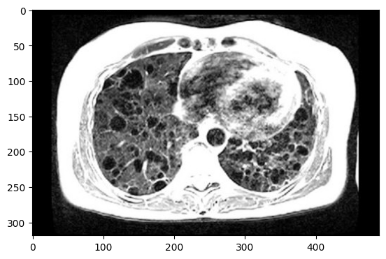

图片来源：https://www.nih.gov/sites/default/files/news-events/news-releases/2019/20191001-nhlbi-lung-th.jpg

        要将图像传递到增强管道，您需要在第 2 步调用 A.Compose 创建的转换函数。在该函数的 image 参数中，您需要传递要增强的图像。

#transform will return a dictionary with a single key image. 
#Value at that key will contain an augmented image.
transformed = transform(image=image)
transformed_image = transformed["image"]
cv2_imshow(transformed_image)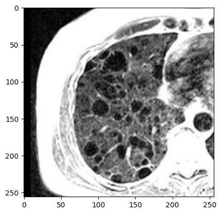

让我们在上面的肺部 MRI 图像上看到更多转换

import os
import random
import albumentations as A
import cv2
import numpy as np
from matplotlib import pyplot as plt
from skimage.color import label2rgb


BOX_COLOR = (255, 0, 0) # Red
TEXT_COLOR = (255, 255, 255) # White

#function to visualize bounding box
#The visualization function is based on 
#https://github.com/facebookresearch/Detectron/blob/master/detectron/utils/vis.py
def visualize_bbox(img, bbox, color=BOX_COLOR, thickness=2, **kwargs):
    x_min, y_min, w, h = bbox
    x_min, x_max, y_min, y_max = int(x_min), int(x_min + w), int(y_min), int(y_min + h)
    cv2.rectangle(img, (x_min, y_min), (x_max, y_max), color=color, thickness=thickness)
    return img
#function to display title text
def visualize_titles(img, bbox, title, font_thickness = 2, font_scale=0.35, **kwargs):
    x_min, y_min = bbox[:2]
    x_min = int(x_min)
    y_min = int(y_min)
    ((text_width, text_height), _) = cv2.getTextSize(title, cv2.FONT_HERSHEY_SIMPLEX, 
                                                     font_scale, font_thickness)
    cv2.rectangle(img, (x_min, y_min - int(1.3 * text_height)), 
                  (x_min + text_width, y_min), BOX_COLOR, -1)
    cv2.putText(img, title, (x_min, y_min - int(0.3 * text_height)), 
                cv2.FONT_HERSHEY_SIMPLEX, font_scale, TEXT_COLOR,
                font_thickness, lineType=cv2.LINE_AA)
    return img

#function to apply transforms and display transformed images
def augment_and_show(aug, image, mask=None, bboxes=[], categories=[], 
                     category_id_to_name=[], filename=None,
                     font_scale_orig=0.35, font_scale_aug=0.35, show_title=True, **kwargs):

    if mask is None:
        augmented = aug(image=image, bboxes=bboxes, category_ids=categories)
    else:
        augmented = aug(image=image, mask=mask, bboxes=bboxes, category_ids=categories)

    image = cv2.cvtColor(image, cv2.COLOR_BGR2RGB)
    image_aug = cv2.cvtColor(augmented['image'], cv2.COLOR_BGR2RGB)

    for bbox in bboxes:
        visualize_bbox(image, bbox, **kwargs)

    for bbox in augmented['bboxes']:
        visualize_bbox(image_aug, bbox, **kwargs)

    if show_title:
        for bbox,cat_id in zip(bboxes, categories):
            visualize_titles(image, bbox, category_id_to_name[cat_id],
                             font_scale=font_scale_orig, **kwargs)
        for bbox,cat_id in zip(augmented['bboxes'], augmented['category_ids']):
            visualize_titles(image_aug, bbox, 
                             category_id_to_name[cat_id], font_scale=font_scale_aug, **kwargs)


    if mask is None:
        f, ax = plt.subplots(1, 2, figsize=(16, 8))

        ax[0].imshow(image)
        ax[0].set_title('Original image')

        ax[1].imshow(image_aug)
        ax[1].set_title('Augmented image')
    else:
        f, ax = plt.subplots(2, 2, figsize=(16, 16))

        if len(mask.shape) != 3:
            mask = label2rgb(mask, bg_label=0)
            mask_aug = label2rgb(augmented['mask'], bg_label=0)
        else:
            mask = cv2.cvtColor(mask, cv2.COLOR_BGR2RGB)
            mask_aug = cv2.cvtColor(augmented['mask'], cv2.COLOR_BGR2RGB)

        ax[0, 0].imshow(image)
        ax[0, 0].set_title('Original image')

        ax[0, 1].imshow(image_aug)
        ax[0, 1].set_title('Augmented image')

        ax[1, 0].imshow(mask, interpolation='nearest')
        ax[1, 0].set_title('Original mask')

        ax[1, 1].imshow(mask_aug, interpolation='nearest')
        ax[1, 1].set_title('Augmented mask')

    f.tight_layout()

    if filename is not None:
        f.savefig(filename)

    if mask is None:
        return augmented['image'], None, augmented['bboxes']

    return augmented['image'], augmented['mask'], augmented['bboxes']

#helper function to find a filename in a directory
def find_in_dir(dirname):
    return [os.path.join(dirname, fname) for fname in sorted(os.listdir(dirname))]

image = cv2.imread('lung_mri.jpg')


random.seed(42)

bbox_params = A.BboxParams(format='coco', label_fields=['category_ids'])

light = A.Compose([
    A.RandomBrightnessContrast(p=1),
    A.RandomGamma(p=1),
    A.CLAHE(p=1),
], p=1, bbox_params=bbox_params)

medium = A.Compose([
    A.CLAHE(p=1),
    A.HueSaturationValue(hue_shift_limit=20, sat_shift_limit=50, val_shift_limit=50, p=1),
], p=1, bbox_params=bbox_params)


strong = A.Compose([
    A.RGBShift(p=1),
     A.Blur(p=1),
     A.GaussNoise(p=1),
     A.ElasticTransform(p=1),
], p=1, bbox_params=bbox_params)



r = augment_and_show(light, image)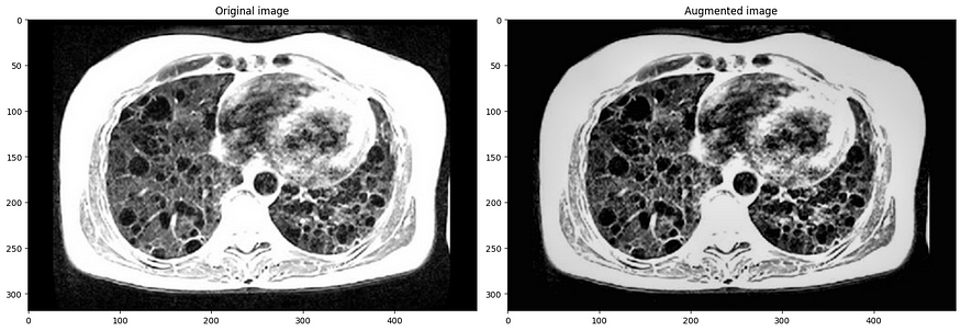

r = augment_and_show(medium, image)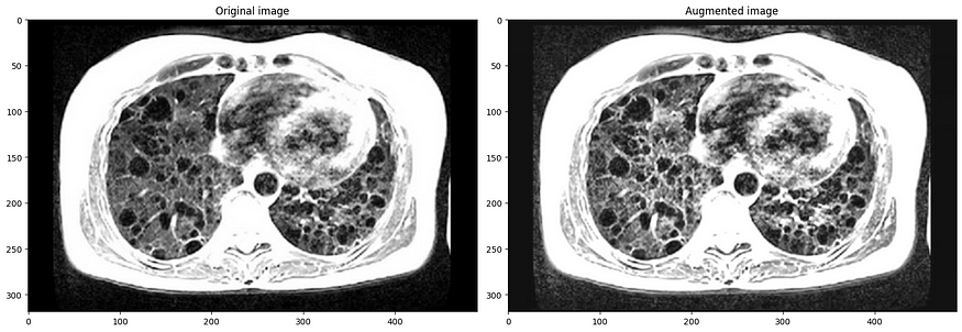

 r  = augment_and_show(strong, image)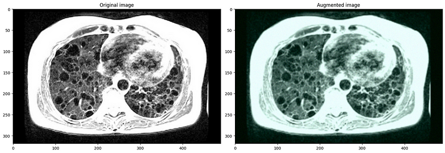 

2.3 在albumentations库中实现的所有像素级变换

        这些转换在像素级别应用于输入图像，并返回任何其他输入目标，如蒙版、边界框或关键点，保持不变。

• 高级模糊
• 模糊
• 克拉赫
• 频道辍学
• ChannelShuffle （频道随机播放）
• 色差
• 颜色抖动
• 离 焦
• 缩小规模
• 浮雕
• 等化
• 美国食品药品监督管理局
• 花式PCA
• FromFloat （从浮点数）
• GaussNoise （高斯噪声）
• GaussianBlur （高斯模糊）
• 玻璃模糊
• 直方图匹配
• HueSaturationValue
• ISO 诺伊斯
• 图像压缩
• InvertImg （反转图像）
• 中值模糊
• 运动模糊
• MultiplicativeNoise （乘法噪声）
• 正常化
• PixelDistributionAdaptation 像素分布适应
• PlanckianJitter
• 色调分离
• RGBShift
• RandomBrightnessContrast （随机亮度对比度）
• RandomFog （随机雾）
• 随机伽玛
• 随机砾石
• 随机雨
• RandomShadow （随机阴影）
• 随机雪
• 随机太阳耀斑
• 随机音调曲线
• 振铃过冲
• 提高
• 曝光
• 飞溅
• 超像素
• 模板转换
• 文本图像
• ToFloat 浮点数
• 到 Gray
• ToRGB
• 棕榈
• UnsharpMask （取消锐化蒙版）
• 缩放模糊

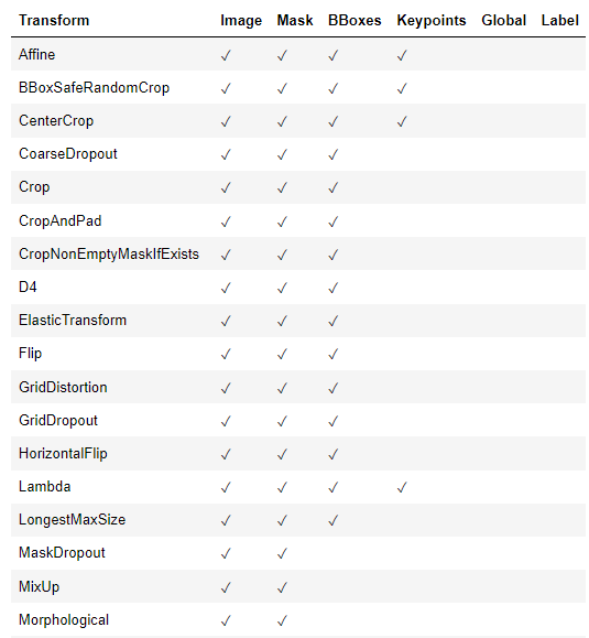
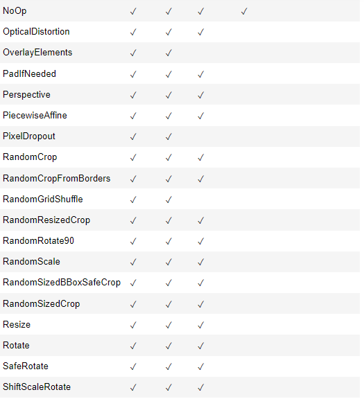
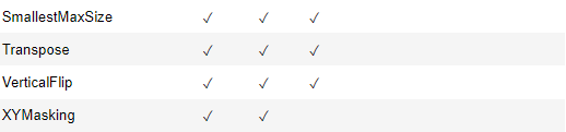
2.4 空间级转换

        下面给出了它们支持的空间级变换和目标。如果尝试将空间级转换应用于不受支持的目标，则 Albumentations 将引发错误。

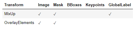
2.5 混合级别转换

        将多个图像混合为一个图像的转换

三、让我们看看上述实现中的转换。

## Simple Augmentations
import random
import cv2
from matplotlib import pyplot as plt
import albumentations as A


def visualize(image):
    plt.figure(figsize=(10, 10))
    plt.axis('off')
    plt.imshow(image)


image = cv2.imread('dog_image.png')
image = cv2.cvtColor(image, cv2.COLOR_BGR2RGB)
visualize(image)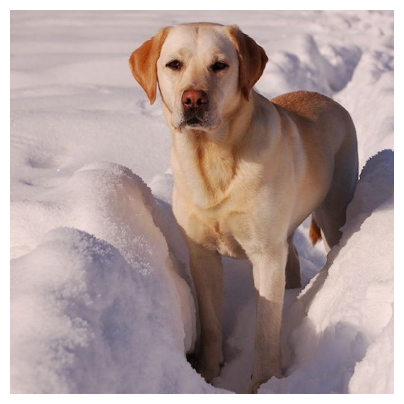

图片来源：https://github.com/albumentations-team/albumentations_examples/

定义一个增强，将图像传递给它并接收增强图像 我们修复随机种子以进行可视化，因此增强将始终产生相同的结果。在实际的计算机视觉管道中，在对图像应用转换之前，不应修复随机种子，因为在这种情况下，管道将始终输出相同的图像。图像增强的目的是每次使用不同的转换。

transform = A.HorizontalFlip(p=0.5)
random.seed(7)
augmented_image = transform(image=image)['image']
visualize(augmented_image)

transform = A.ShiftScaleRotate(p=0.5)
random.seed(7)
augmented_image = transform(image=image)['image']
visualize(augmented_image)

#Define an augmentation pipeline using Compose, pass the image to it and receive the augmented image

transform = A.Compose([
    A.CLAHE(),
    A.RandomRotate90(),
    A.Transpose(),
    A.ShiftScaleRotate(shift_limit=0.0625, scale_limit=0.50, rotate_limit=45, p=.75),
    A.Blur(blur_limit=3),
    A.OpticalDistortion(),
    A.GridDistortion(),
    A.HueSaturationValue(),
])
random.seed(42)
augmented_image = transform(image=image)['image']
visualize(augmented_image)

transform = A.Compose([
        A.RandomRotate90(),
        A.Flip(),
        A.Transpose(),
        A.GaussNoise(),
        A.OneOf([
            A.MotionBlur(p=.2),
            A.MedianBlur(blur_limit=3, p=0.1),
            A.Blur(blur_limit=3, p=0.1),
        ], p=0.2),
        A.ShiftScaleRotate(shift_limit=0.0625, scale_limit=0.2, rotate_limit=45, p=0.2),
        A.OneOf([
            A.OpticalDistortion(p=0.3),
            A.GridDistortion(p=.1),
        ], p=0.2),
        A.OneOf([
            A.CLAHE(clip_limit=2),
            A.RandomBrightnessContrast(),
        ], p=0.3),
        A.HueSaturationValue(p=0.3),
    ])
random.seed(42)
augmented_image = transform(image=image)['image']
visualize(augmented_image)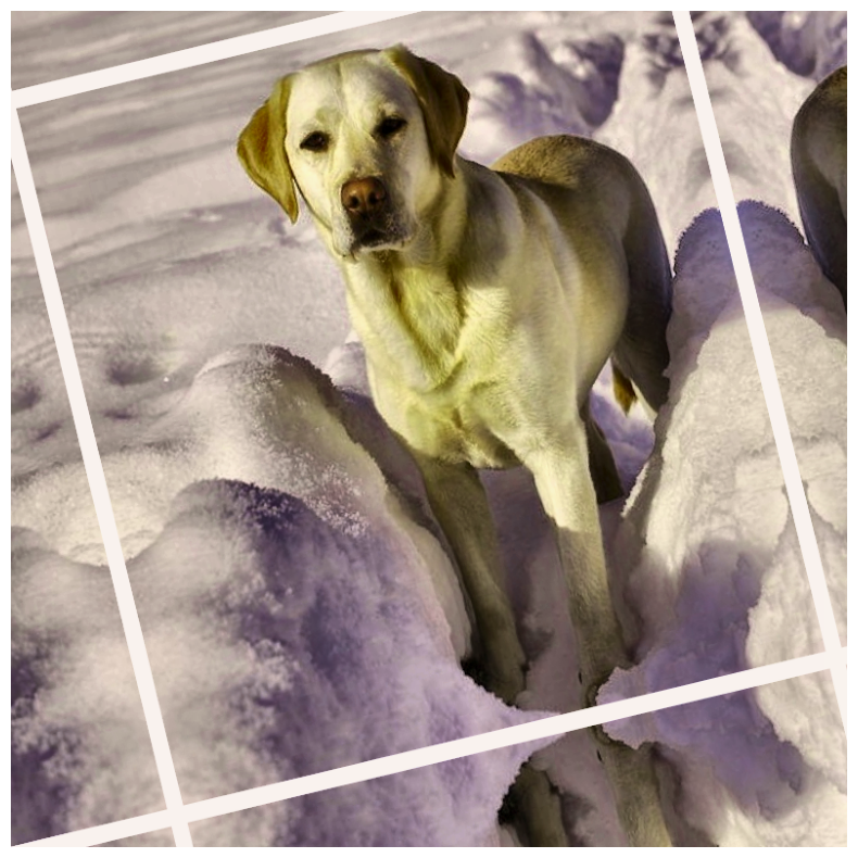

3.1 在专辑中实现的天气相关转换

import random 
import cv2 
from matplotlib import pyplot as plt 
import albumentations as A


def visualize(image):
    #image = cv2.cvtColor(image, cv2.COLOR_BGR2RGB)
    plt.figure(figsize=(20, 10))
    plt.axis('off')
    plt.imshow(image)

image = cv2.imread('weather_example.jpg')
image = cv2.cvtColor(image, cv2.COLOR_BGR2RGB)
visualize(image)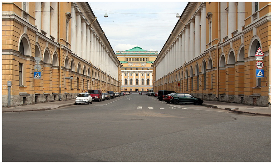

3.2 随机雨

        我们修复随机种子以达到可视化目的，因此增强将始终产生相同的结果。在实际的计算机视觉管道中，在对图像应用转换之前，不应修复随机种子，因为在这种情况下，管道将始终输出相同的图像。图像增强的目的是每次使用不同的转换。

transform = A.Compose([A.RandomRain(brightness_coefficient=0.9, drop_width=1, blur_value=5, p=1)],)
#random.seed(7)
transformed = transform(image=image)
visualize(transformed['image'])

#RandomSnow

transform = A.Compose(
    [A.RandomSnow(brightness_coeff=2.5, snow_point_lower=0.3, snow_point_upper=0.5, p=1)],
)
random.seed(7)
transformed = transform(image=image)
visualize(transformed['image'])

#RandomSunFlare

transform = A.Compose(
    [A.RandomSunFlare(flare_roi=(0, 0, 1, 0.5), angle_lower=0.5, p=1)],
)
random.seed(7)
transformed = transform(image=image)
visualize(transformed['image'])

#RandomShadow

transform = A.Compose(
    [A.RandomShadow(num_shadows_lower=1, num_shadows_upper=1, shadow_dimension=5, shadow_roi=(0, 0.5, 1, 1), p=1)],
)
random.seed(7)
transformed = transform(image=image)
visualize(transformed['image'])

#RandomFog

transform = A.Compose(
    [A.RandomFog(fog_coef_lower=0.7, fog_coef_upper=0.8, alpha_coef=0.1, p=1)],
)
random.seed(7)
transformed = transform(image=image)
visualize(transformed['image'])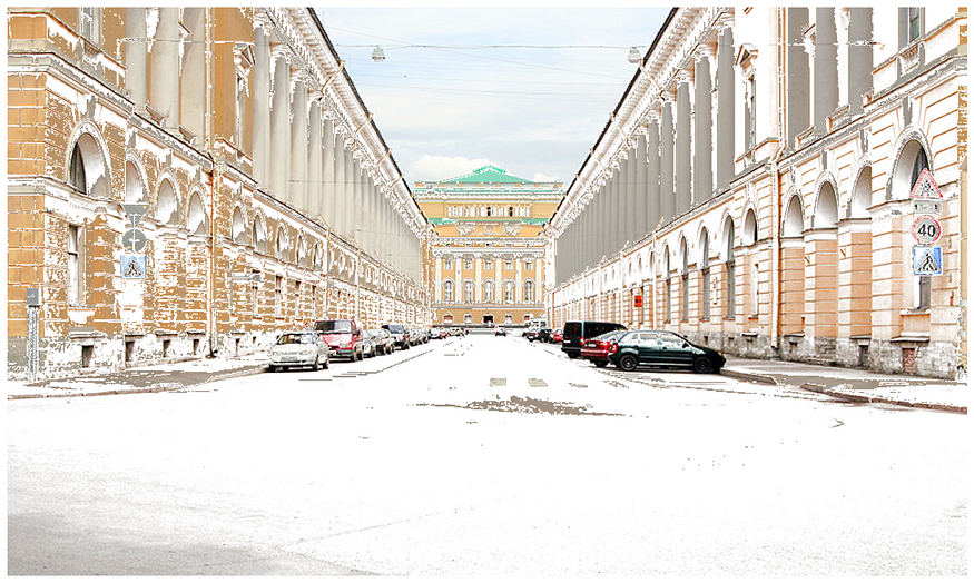

随机雪变换

3.3 在相册中处理非 8 位图像

        例如 16 位 TIFF 图像。卫星影像中使用 16 位影像。以下技术可应用于所有非 8 位图像（即 24 位图像、32 位图像等）。

import random
import cv2
from matplotlib import pyplot as plt
import albumentations as A


#visualize function will be a bit different for TIFF images
import numpy as np
def visualize(image):
    # Divide all values by 65535 so we can display the image using matplotlib
    image = image / np.max(image)
    plt.figure(figsize=(10, 10))
    plt.axis('off')
    plt.imshow(image)


#Read the 16-bit TIFF image from the disk
# The image is taken from http://www.brucelindbloom.com/index.html?ReferenceImages.html
# © Bruce Justin Lindbloom
image = cv2.imread('DeltaE_16bit_gamma2.2.tif', cv2.IMREAD_UNCHANGED)
image = cv2.cvtColor(image, cv2.COLOR_BGR2RGB)
visualize(image)

transform = A.Compose([
    A.ToFloat(max_value=65535.0),

    A.RandomRotate90(),
    A.Flip(),
    A.OneOf([
        A.MotionBlur(p=0.2),
        A.MedianBlur(blur_limit=3, p=0.1),
        A.Blur(blur_limit=3, p=0.1),
    ], p=0.2),
    A.ShiftScaleRotate(shift_limit=0.0625, scale_limit=0.2, 
                       rotate_limit=45, p=0.2),
    A.OneOf([
        A.OpticalDistortion(p=0.3),
        A.GridDistortion(p=0.1),
    ], p=0.2),
    A.HueSaturationValue(hue_shift_limit=20, sat_shift_limit=0.1, 
                         val_shift_limit=0.1, p=0.3),

    A.FromFloat(max_value=65535.0),
])

random.seed(7)
augmented = transform(image=image)
visualize(augmented['image'])

3.4 在文档图像中增强文本（叠加元素）

        管道处理 TIFF 图像和关联的 JSON 文件，这些文件描述文档图像中的文本行及其边界框 GitHub - danaaubakirova/doc-augmentation

import cv2
from matplotlib import pyplot as plt
from PIL import ImageDraw, ImageFont, Image
from pylab import *
import albumentations as A
import json


def visualize(image):
    plt.figure(figsize=(20, 10))
    plt.axis('off')
    plt.imshow(image)

def load_rgb(image_path):
    image = cv2.imread(image_path)
    return cv2.cvtColor(image, cv2.COLOR_BGR2RGB)

font_path = "LiberationSerif-Regular.ttf"
image = load_rgb("docs.png")

with open("text.json") as f:
    labels = json.load(f)
visualize(image)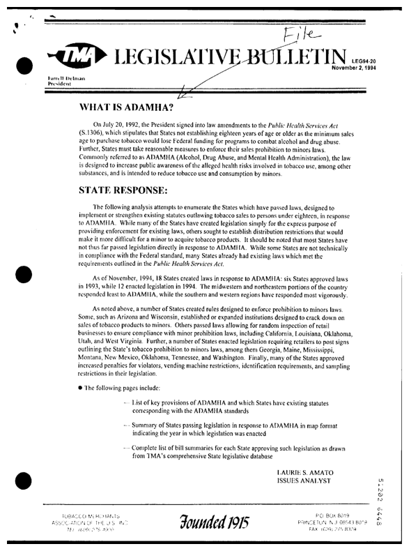

transform = A.Compose([A.OverlayElements(p=1)])


def render_text(bbox_shape, text, font):
    bbox_height, bbox_width = bbox_shape

    # Create an empty RGB image with the size of the bounding box
    bbox_img = Image.new("RGB", (bbox_width, bbox_height), color="white")
    draw = ImageDraw.Draw(bbox_img)

    # Draw the text in red
    draw.text((0, 0), text, fill="red", font=font)

    return np.array(bbox_img)




bbox_indices_to_update = np.random.choice(range(len(labels["text"])), 10)
labels.keys()

image_height, image_width = image.shape[:2]
num_channels = image.shape[2] if len(image.shape) == 3 else 1


metadata = []
for index in bbox_indices_to_update:
    selected_bbox = labels["bbox"][index]

    # You may apply any transforms you want to text like 
    #random deletion, swapping words, applying synonims, etc
    text = labels["text"][index]

    left, top, width_norm, height_norm = selected_bbox

    bbox_height = int(image_height * height_norm)
    bbox_width = int(image_width * width_norm)

    font = ImageFont.truetype(font_path, int(0.90 * bbox_height))

    overlay_image = render_text((bbox_height, bbox_width), text, font)

    metadata += [
        {
            "image": overlay_image,
            "bbox": (left, top, left + width_norm, top + height_norm)
        }
    ]


transformed = transform(image=image, overlay_metadata=metadata)
visualize(transformed["image"])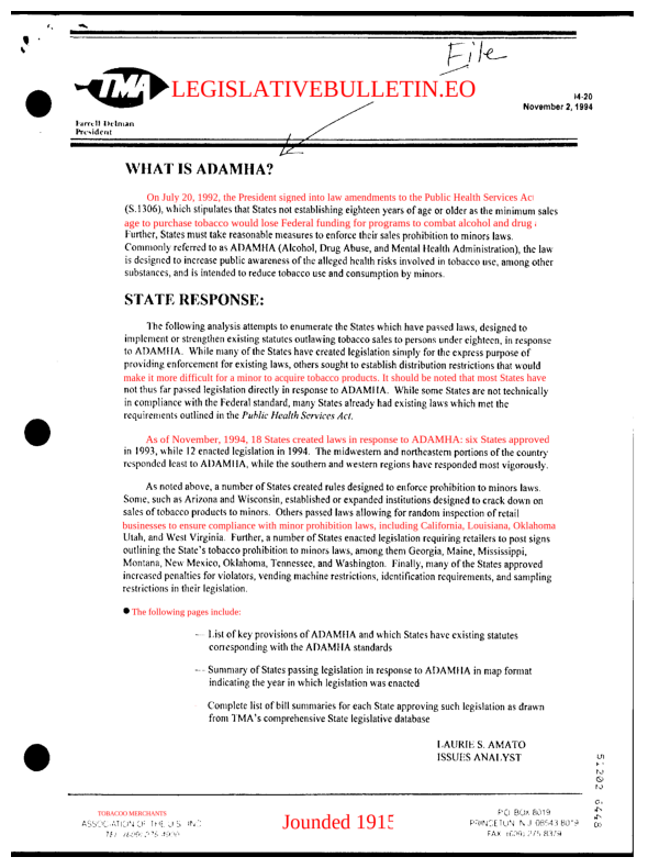

transform_complex = A.Compose([A.OverlayElements(p=1),
                               A.RandomCrop(p=1, height=1024, width=1024),
                               A.PlanckianJitter(p=1),
                               A.Affine(p=1)
                              ])
transformed = transform_complex(image=image, overlay_metadata=metadata)
visualize(transformed["image"])

3.5 带相册的边界框关键点旋转

from typing import List
import albumentations as A
import cv2
import matplotlib.pyplot as plt
import numpy as np


def visualize(image: np.ndarray, keypoints: List[List[float]], 
              bboxes: List[List[float]]) -> np.ndarray:
    overlay = image.copy()
    for kp in keypoints:
        cv2.circle(overlay, (int(kp[0]), int(kp[1])), 20, 
                   (0, 200, 200), thickness=2, lineType=cv2.LINE_AA)

    for box in bboxes:
        cv2.rectangle(overlay, (int(box[0]), int(box[1])), 
                      (int(box[2]), int(box[3])), (200, 0, 0), thickness=2)

    return overlay


def main() -> None:
    image = cv2.imread("image_1.jpg")

    keypoints = cv2.goodFeaturesToTrack(
        cv2.cvtColor(image, cv2.COLOR_RGB2GRAY), maxCorners=100, 
        qualityLevel=0.5, minDistance=5
    ).squeeze(1)

    bboxes = [(kp[0] - 10, kp[1] - 10, kp[0] + 10, kp[1] + 10) for kp in keypoints]

    disp_image = visualize(image, keypoints, bboxes)
    plt.figure(figsize=(10, 10))
    plt.imshow(cv2.cvtColor(disp_image, cv2.COLOR_RGB2BGR))
    plt.tight_layout()
    plt.show()

    aug = A.Compose(
        [A.ShiftScaleRotate(scale_limit=0.1, shift_limit=0.2, 
                            rotate_limit=10, always_apply=True)],
        bbox_params=A.BboxParams(format="pascal_voc", label_fields=["bbox_labels"]),
        keypoint_params=A.KeypointParams(format="xy"),
    )

    for _i in range(10):
        data = aug(image=image, keypoints=keypoints, bboxes=bboxes, 
                   bbox_labels=np.ones(len(bboxes)))

        aug_image = data["image"]
        aug_image = visualize(aug_image, data["keypoints"], data["bboxes"])

        plt.figure(figsize=(10, 10))
        plt.imshow(cv2.cvtColor(aug_image, cv2.COLOR_RGB2BGR))
        plt.tight_layout()
        plt.show()

if __name__ == "__main__":
    main()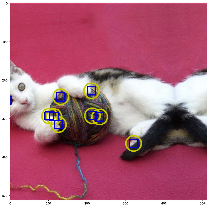

3.6 绘制边界框

import random
import cv2
from matplotlib import pyplot as plt
import albumentations as A

可视化功能基于 Detectron/detectron/utils/vis.py at main · facebookresearch/Detectron · GitHub

BOX_COLOR = (255, 0, 0) # Red
TEXT_COLOR = (255, 255, 255) # White


def visualize_bbox(img, bbox, class_name, color=BOX_COLOR, thickness=2):
    """Visualizes a single bounding box on the image"""
    x_min, y_min, w, h = bbox
    x_min, x_max, y_min, y_max = int(x_min), int(x_min + w), int(y_min), int(y_min + h)

    cv2.rectangle(img, (x_min, y_min), (x_max, y_max), color=color, thickness=thickness)

    ((text_width, text_height), _) = cv2.getTextSize(class_name, cv2.FONT_HERSHEY_SIMPLEX, 0.35, 1)
    cv2.rectangle(img, (x_min, y_min - int(1.3 * text_height)), 
                  (x_min + text_width, y_min), BOX_COLOR, -1)
    cv2.putText(
        img,
        text=class_name,
        org=(x_min, y_min - int(0.3 * text_height)),
        fontFace=cv2.FONT_HERSHEY_SIMPLEX,
        fontScale=0.35,
        color=TEXT_COLOR,
        lineType=cv2.LINE_AA,
    )
    return img


def visualize(image, bboxes, category_ids, category_id_to_name):
    img = image.copy()
    for bbox, category_id in zip(bboxes, category_ids):
        class_name = category_id_to_name[category_id]
        img = visualize_bbox(img, bbox, class_name)
    plt.figure(figsize=(12, 12))
    plt.axis('off')
    plt.imshow(img)

在此示例中，我们将使用 COCO 数据集中的图像，该图像具有两个关联的边界框。该图片可在 COCO - Common Objects in Context

image = cv2.imread('000000386298.jpg')
image = cv2.cvtColor(image, cv2.COLOR_BGR2RGB)

3.7 定义两个带有坐标和类标签的边界框

        这些边界框的坐标使用 coco 格式声明。每个边界框都使用四个值 [x_min、y_min、宽度、高度] 进行描述。关于边界框坐标不同格式的详细说明，请参考 边界框 — Bounding boxes augmentation for object detection - Albumentations Documentation 的文档文章。

bboxes = [[5.66, 138.95, 147.09, 164.88], [366.7, 80.84, 132.8, 181.84]]
category_ids = [17, 18]

# We will use the mapping from category_id to the class name
# to visualize the class label for the bounding box on the image
category_id_to_name = {17: 'cat', 18: 'dog'}


#Visuaize the original image with bounding boxes
visualize(image, bboxes, category_ids, category_id_to_name)

四、定义增强管道

        要创建适用于边界框的增强管道，您需要将 BboxParams 的一个实例传递给 Compose。在 BboxParams 中，您需要指定边界框的坐标格式以及可选的一些其他参数。有关 BboxParams 的详细说明，请参阅有关边界框 — Bounding boxes augmentation for object detection - Albumentations Documentation 的文档文章。

transform = A.Compose(
    [A.HorizontalFlip(p=0.5)],
    bbox_params=A.BboxParams(format='coco', label_fields=['category_ids']),
)



random.seed(7)
transformed = transform(image=image, bboxes=bboxes, category_ids=category_ids)
visualize(
    transformed['image'],
    transformed['bboxes'],
    transformed['category_ids'],
    category_id_to_name,
)

transform = A.Compose(
    [A.ShiftScaleRotate(p=0.5)],
    bbox_params=A.BboxParams(format='coco', label_fields=['category_ids']),
)

random.seed(7)
transformed = transform(image=image, bboxes=bboxes, category_ids=category_ids)
visualize(
    transformed['image'],
    transformed['bboxes'],
    transformed['category_ids'],
    category_id_to_name,
)

#Define a complex augmentation piepline

transform = A.Compose([
        A.HorizontalFlip(p=0.5),
        A.ShiftScaleRotate(p=0.5),
        A.RandomBrightnessContrast(p=0.3),
        A.RGBShift(r_shift_limit=30, g_shift_limit=30, b_shift_limit=30, p=0.3),
    ],
    bbox_params=A.BboxParams(format='coco', label_fields=['category_ids']),
)

random.seed(7)
transformed = transform(image=image, bboxes=bboxes, category_ids=category_ids)
visualize(
    transformed['image'],
    transformed['bboxes'],
    transformed['category_ids'],
    category_id_to_name,
)

4.1 min_area和min_visibility参数

        如果应用空间增强，则边界框的大小可能会更改，例如，在裁剪图像的一部分或调整图像大小时。

        min_area 和 min_visibility 参数控制 Albumentations 应对增强的边界框执行的操作，如果其大小在增强后发生了变化。如果应用空间增强，则边界框的大小可能会更改，例如，在裁剪图像的一部分或调整图像大小时。

        min_area 是以像素为单位的值。如果增强后边界框的面积小于 min_area，则 Albumentations 将删除该框。因此，返回的增强边界框列表将不包含该边界框。

min_visibility 是介于 0 和 1 之间的值。如果增强后的边界框区域与增强前的边界框面积之比小于 min_visibility，则 Albumentations 将丢弃该框。因此，如果增强过程切掉了大部分边界框，则该框将不会出现在返回的增强边界框列表中。

4.2 使用 min_area 和 min_visibilty 的默认值定义增强管道

如果不传递 min_area 和 min_visibility 参数，则 Albumentations 将使用 0 作为它们的默认值。

transform = A.Compose(
    [A.CenterCrop(height=280, width=280, p=1)],
    bbox_params=A.BboxParams(format='coco', label_fields=['category_ids']),
)

transformed = transform(image=image, bboxes=bboxes, category_ids=category_ids)
visualize(
    transformed['image'],
    transformed['bboxes'],
    transformed['category_ids'],
    category_id_to_name,
)

五、从数学模型对变换分类

5.1 半音差

import cv2
from matplotlib import pyplot as plt
import cv2

import albumentations as A

def visualize(image):
    plt.figure(figsize=(10, 5))
    plt.axis('off')
    plt.imshow(image)

def load_rgb(image_path):
    image = cv2.imread(image_path)
    return cv2.cvtColor(image, cv2.COLOR_BGR2RGB)


img_path = "alina_rossoshanska.jpeg"
img = load_rgb(img_path)
visualize(img)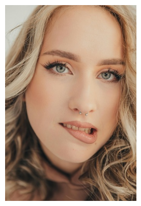

#Red-blue mode

transform = A.Compose([A.ChromaticAberration(mode="red_blue", 
                                             primary_distortion_limit=0.5, 
                                             secondary_distortion_limit=0.1, p=1)])

plt.figure(figsize=(15, 10))

num_images = 12

# Loop through the list of images and plot them with subplot
for i in range(num_images):
    transformed_image = transform(image = img)["image"]
    plt.subplot(4, 3, i + 1)
    plt.imshow(transformed_image)
    plt.axis('off')

plt.tight_layout()
plt.show()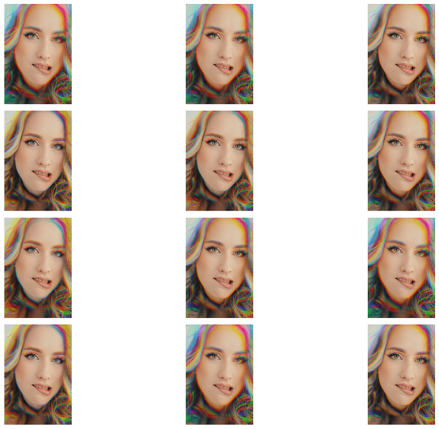

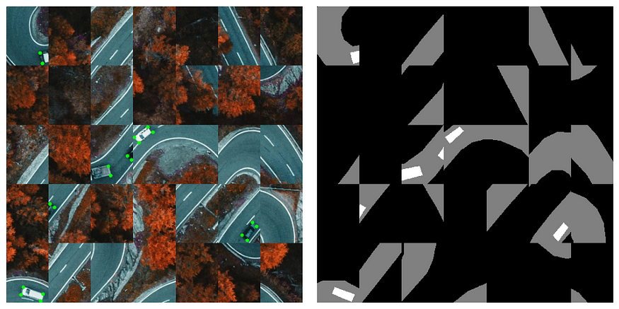
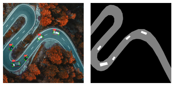
5.2 D4 变换

        Geomatric 变换是使用最广泛的增强。主要是因为他们没有在原始数据分布之外获取数据，并且因为他们有直觉”。

D4 变换将原始图像映射到 8 种状态之一。

• e — 身份。原始图像
• r90 — 旋转 90 度
• r180 — 旋转 180 度，等于 v * h = h * v
• r270 — 旋转 270 度
• v — 垂直翻转
• hvt — 跨对角线的反射，等于 t * v * h 或 t * rot180
• h — 水平翻转
• t — 反射活动对角线

相同的转换可以更方便地表示为：

A.Compose（[A.HorizonatalFlip（p=0.5）， A.RandomRotate90（p=1）]）

此变换在影像数据没有首选方向的情况下非常有用：

例如：医学图像、俯视无人机和卫星图像。它适用于：图像、蒙版、关键点、边界框

import json
import hashlib
import random
import numpy as np
import cv2
from matplotlib import pyplot as plt
import albumentations as A



BOX_COLOR = (255, 0, 0)
TEXT_COLOR = (255, 255, 255)
KEYPOINT_COLOR = (0, 255, 0)

def visualize_bbox(img, bbox, class_name, bbox_color=BOX_COLOR, thickness=1):
    """Visualizes a single bounding box on the image"""
    x_min, y_min, x_max, y_max = (int(x) for x in bbox)
    cv2.rectangle(img, (x_min, y_min), (x_max, y_max), 
                  color=bbox_color, thickness=thickness)

    ((text_width, text_height), _) = cv2.getTextSize(class_name, 
                                                     cv2.FONT_HERSHEY_SIMPLEX, 0.35, 1)
    cv2.rectangle(img, (x_min, y_min - int(1.3 * text_height)), 
                  (x_min + text_width, y_min), bbox_color, -1)
    cv2.putText(
        img,
        text=class_name,
        org=(x_min, y_min - int(0.3 * text_height)),
        fontFace=cv2.FONT_HERSHEY_SIMPLEX,
        fontScale=0.35,
        color=TEXT_COLOR,
        lineType=cv2.LINE_AA,
    )
    return img

def vis_keypoints(image, keypoints, color=KEYPOINT_COLOR, diameter=3):
    image = image.copy()
    for (x, y) in keypoints:
        cv2.circle(image, (int(x), int(y)), diameter, color, -1)
    return image

def visualize_one(image, bboxes, keypoints, category_ids, category_id_to_name, mask):
    # Create a copy of the image to draw on
    img = image.copy()

    # Apply each bounding box and corresponding category ID
    for bbox, category_id in zip(bboxes, category_ids):
        class_name = category_id_to_name[category_id]
        img = visualize_bbox(img, bbox, class_name)

    # Apply keypoints if provided
    if keypoints:
        img = vis_keypoints(img, keypoints)

    # Setup plot
    fig, ax = plt.subplots(1, 2, figsize=(6, 3))

    # Show the image with annotations
    ax[0].imshow(img)    
    ax[0].axis('off')

    # Show the mask
    ax[1].imshow(mask, cmap='gray')    
    ax[1].axis('off')

    plt.tight_layout()
    plt.show()

     

def visualize(images, bboxes_list, keypoints_list, 
              category_ids_list, category_id_to_name, masks):
    if len(images) != 8:
        raise ValueError("This function is specifically designed to handle exactly 8 images.")

    num_rows = 4
    num_cols = 4
    
    fig, axs = plt.subplots(num_cols, num_rows, figsize=(20, 20)) 

    for idx, (image, bboxes, keypoints, category_ids, mask) in enumerate(zip(images,
                                                                             bboxes_list, 
                                                                             keypoints_list, 
                                                                             category_ids_list, 
                                                                             masks)):
        img = image.copy()

        # Process each image: draw bounding boxes and keypoints
        for bbox, category_id in zip(bboxes, category_ids):
            class_name = category_id_to_name[category_id]
            img = visualize_bbox(img, bbox, class_name)

        if keypoints:
            img = vis_keypoints(img, keypoints)

        # Calculate subplot indices
        row_index = (idx * 2) // num_rows  # Each pair takes two columns in one row
        col_index_image = (idx * 2) % num_cols  # Image at even index
        col_index_mask = (idx * 2 + 1) % num_cols  # Mask at odd index right after image

        # Plot the processed image
        img_ax = axs[row_index, col_index_image]
        img_ax.imshow(img)        
        img_ax.axis('off')

        # Plot the corresponding mask
        mask_ax = axs[row_index, col_index_mask]
        mask_ax.imshow(mask, cmap='gray')        
        mask_ax.axis('off')

    plt.tight_layout()
    plt.show()

with open("road_labels.json") as f:
    labels = json.load(f)

bboxes = labels["bboxes"]
keypoints = labels["keypoints"]

bgr_image = cv2.imread("road.jpeg")
image = cv2.cvtColor(bgr_image, cv2.COLOR_BGR2RGB)

mask = cv2.imread("road.png", 0)

# In this example we use only one class, hence category_ids is list equal 
#to the number of bounding boxes with only one value
category_ids = [1] * len(labels["bboxes"])
category_id_to_name = {1: "car"}

visualize_one(image, bboxes, keypoints, category_ids, category_id_to_name, mask)

transform = A.Compose([
    A.CenterCrop(height=512, width=256, p=1),
    A.D4(p=1)],
                     bbox_params=A.BboxParams(format='pascal_voc', 
                                              label_fields=['category_ids']),
                     keypoint_params=A.KeypointParams(format='xy'))

transformed = transform(image=image, bboxes=bboxes, 
                        category_ids=category_ids, keypoints=keypoints, mask=mask)

def get_hash(image):
    image_bytes = image.tobytes()
    hash_md5 = hashlib.md5()
    hash_md5.update(image_bytes)    
    return hash_md5.hexdigest()

transformations_dict = {}

for _ in range(80):
    transformed = transform(image=image, bboxes=bboxes, 
                            category_ids=category_ids, keypoints=keypoints, mask=mask)
    image_hash = get_hash(transformed["image"])
    
    if image_hash in transformations_dict:
        transformations_dict[image_hash]['count'] += 1
    else:
        transformations_dict[image_hash] = {
            "count": 1,
            "transformed": transformed
        }

#The transform generates all 8 possible variants with the same probability, including identity transform
len(transformations_dict)

for key in transformations_dict:
    print(key, transformations_dict[key]["count"])

transformed_list = [value["transformed"] for value in transformations_dict.values()]



images = [x["image"] for x in transformed_list]
masks = [x["mask"] for x in transformed_list]
bboxes_list = [x["bboxes"] for x in transformed_list]
keypoints_list = [x["keypoints"] for x in transformed_list]


category_ids_list = [[1] * len(x["bboxes"]) for x in transformed_list]
category_id_to_name = {1: "car"}


visualize(images, bboxes_list, keypoints_list, 
          category_ids_list, category_id_to_name, masks)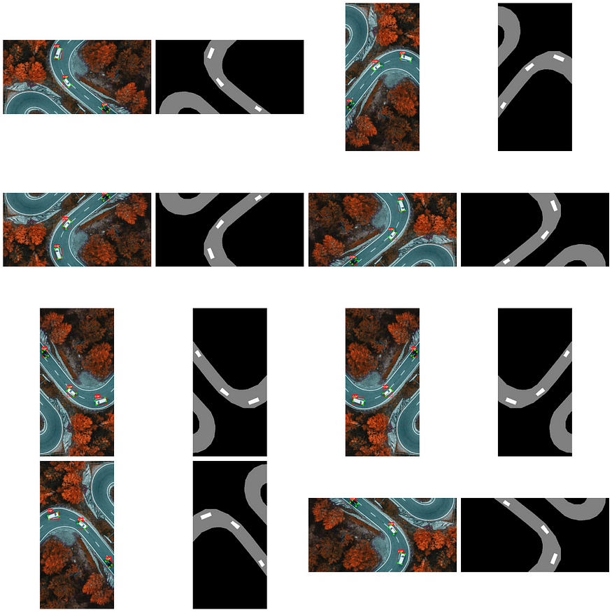

5.3 形态变换

import random

import cv2
from matplotlib import pyplot as plt

import albumentations as A

def visualize(image):
    plt.figure(figsize=(10, 5))
    plt.axis('off')
    plt.imshow(image)

def load_rgb(image_path):
    image = cv2.imread(image_path)
    return cv2.cvtColor(image, cv2.COLOR_BGR2RGB)


img_path = "scan.jpeg"
img = load_rgb(img_path)
visualize(img)

#Dilation expands the white (foreground) regions in a binary or grayscale image.
transform = A.Compose([A.Morphological(p=1, scale=(2, 3), operation='dilation')], p=1)
transformed = transform(image=img)
visualize(transformed["image"])

#Erosion shrinks the white (foreground) regions in a binary or grayscale image.
transform = A.Compose([A.Morphological(p=1, scale=(2, 3), operation='erosion')], p=1)
transformed = transform(image=img)
visualize(transformed["image"])

5.4 域适应转换

DAT 是不使用神经网络的样式迁移。生成的图像看起来并不理想，但可以在合理的时间内动态生成。

import random

import cv2
from matplotlib import pyplot as plt
from pathlib import Path
import numpy as np
import cv2

import albumentations as A

def visualize(image):
    plt.figure(figsize=(10, 5))
    plt.axis('off')
    plt.imshow(image)

def load_rgb(image_path):
    image = cv2.imread(image_path)
    return cv2.cvtColor(image, cv2.COLOR_BGR2RGB)

image1 = load_rgb("park1.png")
image2 = load_rgb("rain2.png")

visualize(image1)

visualize(image2)

5.5 Historgram 匹配

此过程调整输入图像的像素值，使其直方图与参考图像的直方图对齐。在处理多通道图像时，如果输入图像和参考图像的通道数相同，则每个通道的这种对齐都是单独进行的。

transform = A.Compose([A.HistogramMatching(reference_images=[image2], 
                                           read_fn = lambda x: x, 
                                           p=1,
                                           blend_ratio=(0.3, 0.3)
                                          )], p=1)
     
transformed = transform(image=image1)["image"]
visualize(transformed)

5.6 傅里叶域适应 （FDA）

        傅里叶域适应 （FDA） 用于在无监督域适应 （UDA） 的上下文中进行简单的“样式转移”。FDA 操纵图像的频率分量以减少源数据集和目标数据集之间的域差距，有效地使一个域中的图像与另一个域中的图像非常相似，而不会改变其语义内容。

        在训练 （源） 和测试 （目标） 图像来自不同分布的情况下，例如合成图像与真实图像，或昼夜场景，这种转换特别有用。与可能需要复杂对抗训练的传统域适应方法不同，FDA 通过在源图像和目标图像之间交换傅里叶变换的低频分量来实现域对齐。该技术已被证明可以提高模型在目标域上的性能，特别是对于语义分割等任务，而无需对域不变性进行额外的训练。

transform = A.Compose([A.FDA(reference_images=[image1], 
                             read_fn = lambda x: x, p=1, beta_limit=(0.2, 0.2))], p=1)
transformed = transform(image=image1)["image"]
visualize(transformed)

5.7 像素分布

        通过将输入图像的像素值分布与参考图像的像素值分布对齐来执行像素级域自适应。此过程涉及将简单的统计信息（例如 PCA、StandardScaler 或 MinMaxScaler）拟合到原始图像和参考图像，使用在其上训练的变换来转换原始图像，然后使用拟合在参考图像上的变换应用反向变换。其结果是经过改编的图像，它保留了原始内容，同时模仿了参考域的像素值分布。

        该过程可以可视化为两个主要步骤：

• 使用选定的转换将原始图像调整为标准分布空间。
• 通过应用拟合到参考图像上的变换的逆函数，将调整后的图像移动到参考图像的分布空间中。

        该技术在需要协调来自不同领域的图像（例如，合成图像与真实图像、昼夜场景）以在图像处理任务中获得更好的一致性或性能的情况下特别有用。

transform = A.Compose([A.PixelDistributionAdaptation(reference_images=[image1], 
                                                     read_fn = lambda x: x, p=1,  transform_type="pca")], p=1)

transformed = transform(image=image1)["image"]
visualize(transformed)

beta = 0.1

height, width = image1.shape[:2]
border = int(np.floor(min(height, width) * beta))
center_y, center_x = height // 2, width // 2

# Define region for amplitude substitution
y1, y2 = center_y - border, center_y + border

x1, x2 = center_x - border, center_x + border

x1, x2, y1, y2
     
(205, 307, 205, 307)

def low_freq_mutate_np(amp_src, amp_trg, L, h, w):
    b = int(np.floor(min(h, w) * L))
    c_h, c_w = h // 2, w // 2
    h1, h2 = max(0, c_h - b), min(c_h + b, h - 1)
    w1, w2 = max(0, c_w - b), min(c_w + b, w - 1)
    amp_src[h1:h2, w1:w2] = amp_trg[h1:h2, w1:w2]
    return amp_src

def fourier_domain_adaptation(src_img, trg_img, beta=0.1):
    assert src_img.shape == trg_img.shape, "Source and target images must have the same shape."
    src_img = src_img.astype(np.float32)
    trg_img = trg_img.astype(np.float32)

    height, width, num_channels = src_img.shape
    
    # Prepare container for the output image
    src_in_trg = np.zeros_like(src_img)
    
    for c in range(num_channels):
        # Perform FFT on each channel
        fft_src = np.fft.fft2(src_img[:, :, c])
        fft_trg = np.fft.fft2(trg_img[:, :, c])
        
        # Shift the zero frequency component to the center
        fft_src_shifted = np.fft.fftshift(fft_src)
        fft_trg_shifted = np.fft.fftshift(fft_trg)
        
        # Extract amplitude and phase
        amp_src, pha_src = np.abs(fft_src_shifted), np.angle(fft_src_shifted)
        amp_trg = np.abs(fft_trg_shifted)
        
        # Mutate the amplitude part of the source with the target
        
        mutated_amp = low_freq_mutate_np(amp_src.copy(), amp_trg, beta, height, width)
        
        # Combine the mutated amplitude with the original phase
        fft_src_mutated = np.fft.ifftshift(mutated_amp * np.exp(1j * pha_src))
        
        # Perform inverse FFT
        src_in_trg_channel = np.fft.ifft2(fft_src_mutated)
        
        # Store the result in the corresponding channel of the output image
        src_in_trg[:, :, c] = np.real(src_in_trg_channel)
        
    return np.clip(src_in_trg, 0, 255)

visualize(fourier_domain_adaptation(image2, image1, 0.01).astype(np.uint8))

5.8 RandomGridShuffle 随机排序

        此转换将图像划分为网格，然后根据随机映射排列这些网格单元格。

        当只有微特征对模型很重要时，它可能很有用，而记住全局结构可能是有害的。

例如：

• 根据手机后处理算法生成的微伪影（而不是照片的语义特征）来识别用于拍照的手机类型。
• 根据皮肤图像识别压力、葡萄糖、水合作用水平。

import random
import numpy as np
import cv2
from matplotlib import pyplot as plt
import albumentations as A
import json

KEYPOINT_COLOR = (0, 255, 0)

def vis_keypoints(image, keypoints, color=KEYPOINT_COLOR, diameter=3):
    image = image.copy()
    for (x, y) in keypoints:
        cv2.circle(image, (int(x), int(y)), diameter, color, -1)
    return image

def visualize(image, mask, keypoints):
    # Create a copy of the image to draw on
    img = image.copy()

    # Apply keypoints if provided
    if keypoints:
        img = vis_keypoints(img, keypoints)

    # Setup plot
    fig, ax = plt.subplots(1, 2, figsize=(10, 5))

    # Show the image with annotations
    ax[0].imshow(img)    
    ax[0].axis('off')

    # Show the mask
    ax[1].imshow(mask, cmap='gray')    
    ax[1].axis('off')

    plt.tight_layout()
    plt.show()




with open("road_labels.json") as f:
    labels = json.load(f)

keypoints = labels["keypoints"]

bgr_image = cv2.imread("road.jpeg")
image = cv2.cvtColor(bgr_image, cv2.COLOR_BGR2RGB)

mask = cv2.imread("road.png", 0)

visualize(image, mask, keypoints)

transform = A.Compose([A.RandomGridShuffle(grid=(2, 2), p=1)],
                      keypoint_params=A.KeypointParams(format='xy'))
transformed = transform(image=image, keypoints=keypoints, mask=mask)
visualize(transformed["image"], transformed["mask"], transformed["keypoints"])

transform = A.Compose([A.RandomGridShuffle(grid=(3, 3), p=1)], 
                      keypoint_params=A.KeypointParams(format='xy'))
transformed = transform(image=image, keypoints=keypoints, mask=mask)
visualize(transformed["image"], transformed["mask"], transformed["keypoints"])

transform = A.Compose([A.RandomGridShuffle(grid=(5, 7), p=1)],
                      keypoint_params=A.KeypointParams(format='xy'))
transformed = transform(image=image, keypoints=keypoints, mask=mask)
visualize(transformed["image"], transformed["mask"], transformed["keypoints"])

来源：