DDPM pytorch 代码复现

本次只分享代码以及效果，后续更新原理
代码参考 deep_thought

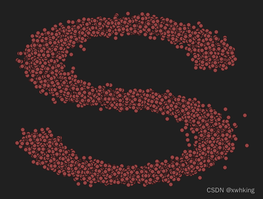
先看动图效果
在这里插入图片描述

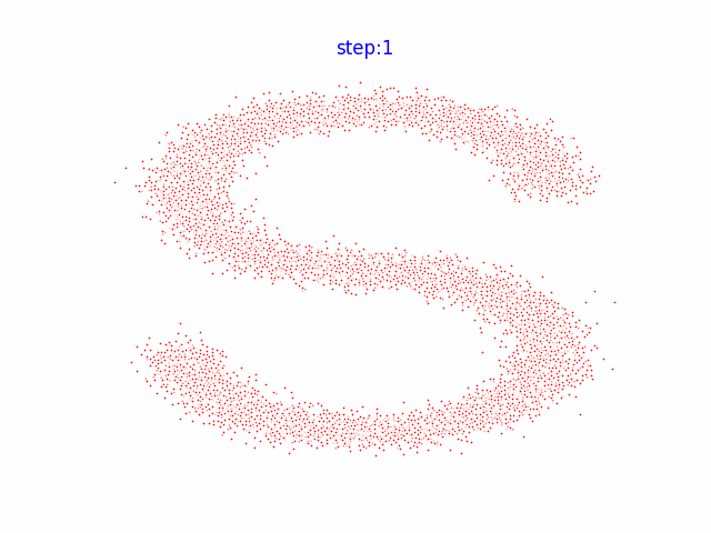
1.选择一个数据集

%matplotlib inline
import matplotlib.pyplot as plt
import numpy as np
from sklearn.datasets import make_s_curve
import torch

s_curve, _ = make_s_curve(10 ** 4, noise=0.1)
s_curve = s_curve[:, [0, 2]] / 10.0

print("shape of moons:", np.shape(s_curve))

data = s_curve.T
fig, ax = plt.subplots()
ax.scatter(*data, color='red', edgecolor='white')

ax.axis('off')

dataset = torch.Tensor(s_curve).float()

在这里插入图片描述

2. 确定超参数

num_steps = 100  # 对于步骤，一开始可以由 被他、分布的均值和标准差来共同确定

# 制定每一步的 beta
betas = torch.linspace(-6, 6, num_steps)
betas = torch.sigmoid(betas) * (0.5e-2 - 1e-5) + 1e-5

# 计算alpha，alpha_prod，alpha_prod_previous、alpha_bar_sqrt等变量的值
alphas = 1 - betas
alphas_prod = torch.cumprod(alphas, 0)
alphas_prod_p = torch.cat([torch.tensor([1]).float(), alphas_prod[:-1]], 0)  # p 表示 previous
alphas_bar_sqrt = torch.sqrt(alphas_prod)
one_minus_alphas_bar_log = torch.log(1 - alphas_prod)
one_minus_alphas_bar_sqrt = torch.sqrt(1 - alphas_prod)

assert alphas.shape == alphas_prod.shape == alphas_prod_p.shape == alphas_bar_sqrt.shape == one_minus_alphas_bar_log.shape == one_minus_alphas_bar_sqrt.shape
print("all the same shape:", betas.shape)

3. 确定扩散过程任意时刻的采样值

# 计算任意时刻的x的采样值，基于x_0核参数重整化技巧
def q_x(x_0, t):
    """可以基于x[0]"得到任意时刻t的x[t]"""
    noise = torch.randn_like(x_0)  # noise 是从正太分布中生成的随机噪声
    alphas_t = alphas_bar_sqrt[t]
    alphas_l_m_t = one_minus_alphas_bar_sqrt[t]
    # alphas_t = extract(alphas_bar_sqrt,t,x_0) # 得到sqrt(alphas_bar[t]),x_0的作用是传入shape
    # alphas_l_m_t = extract(one_minus_alphas_bar_sqrt,t,x_0) # 得到sqrt（1-alphas_bar[t])
    return (alphas_t * x_0 + alphas_l_m_t * noise)  # 在 x[0]基础上添加噪声

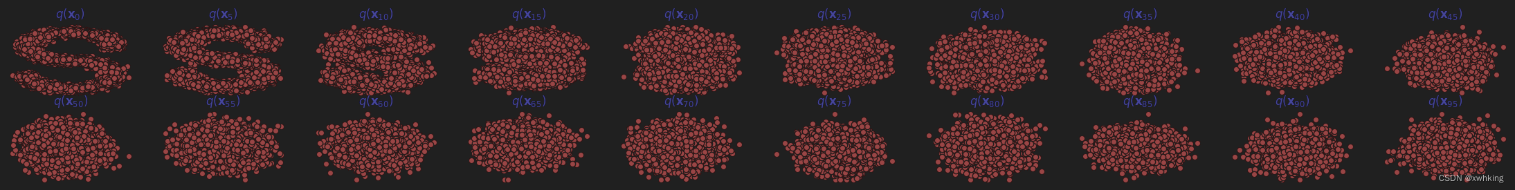
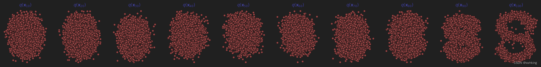
4.演示原始数据分布加噪 100 步后的效果

num_shows = 20
fig, axs = plt.subplots(2, 10, figsize=(28, 3))
plt.rc('text', color='blue')
# 共有 10000 个点，每个点包含两个坐标
# 生成 100 步以内每隔 5 步加噪声的图像
for i in range(num_shows):
    j = i // 10
    k = i % 10
    q_i = q_x(dataset, torch.tensor([i * num_steps // num_shows]))  # 生成 t 时刻的采样数据
    axs[j, k].scatter(q_i[:, 0], q_i[:, 1], color='red', edgecolors='white')

    axs[j, k].set_axis_off()
    axs[j, k].set_title('$q(\mathbf{x}_{' + str(i * num_steps // num_shows) + '})$')

在这里插入图片描述

5. 编写拟合扩散过程高斯分布的模型


import torch
import torch.nn as nn


class MLPDiffusion(nn.Module):
    def __init__(self, n_steps, num_units=128):
        super(MLPDiffusion, self).__init__()
        self.linears = nn.ModuleList([
            nn.Linear(2, num_units),
            nn.ReLU(),
            nn.Linear(num_units, num_units),
            nn.ReLU(),
            nn.Linear(num_units, num_units),
            nn.ReLU(),
            nn.Linear(num_units, 2)
        ])
        self.step_embeddings = nn.ModuleList(
            [
                nn.Embedding(n_steps, num_units),
                nn.Embedding(n_steps, num_units),
                nn.Embedding(n_steps, num_units),
            ]
        )

    def forward(self, x_0, t):
        x = x_0
        for idx, embedding_layer in enumerate(self.step_embeddings):
            t_embedding = embedding_layer(t)
            x = self.linears[2 * idx](x)
            x += t_embedding
            x = self.linears[2 * idx + 1](x)

        x = self.linears[-1](x)

        return x

6.编写训练的误差函数

def diffusion_loss_fn(model, x_0, alphas_bar_sqrt, one_minus_alphas_bar_sqrt, n_steps):
    """对任意时刻t进行采样计算loss"""
    batch_size = x_0.shape[0]

    # 随机采样一个时刻t，为了提高训练效率，这里确保 t 不重复
    # weights = torch.ones(n_steps).expand(batch_size,-1)
    # t = torch.multinomial(weights,num_samples=1,replacement=False) # [batch_size,1]
    t = torch.randint(0, n_steps, size=(batch_size // 2,))
    t = torch.cat([t, n_steps - 1 - t], dim=0)
    t = t.unsqueeze(-1)
    # print(t.shape)

    # x0 的系数
    a = alphas_bar_sqrt[t]

    # eps的系数
    aml = one_minus_alphas_bar_sqrt[t]

    # 生成随机噪声eps
    e = torch.randn_like(x_0)

    # 构造模型的输入
    x = x_0 * a + e * aml

    # 送入模型，得到 t 时刻的随机噪声预测值
    output = model(x, t.squeeze(-1))

    # 与真实噪声一起计算误差，求平均值
    return (e - output).square().mean()

7.编写逆扩散采样函数

def p_sample_loop(model, shape, n_steps, betas, one_minus_alphas_bar_sqrt):
   """ 从x[T]恢复x[T-1],x[t-2]...x[0]"""
   cur_x = torch.randn(shape)
   x_seq = [cur_x]
   for i in reversed(range(n_steps)):
       cur_x = p_sample(model, cur_x, i, betas, one_minus_alphas_bar_sqrt)
       x_seq.append(cur_x)
   return x_seq


def p_sample(model, x, t, betas, one_minus_alphas_bar_sqrt):
   """从x[T]采样 t 时刻的重构值"""

   t = torch.tensor([t])

   coeff = betas[t] / one_minus_alphas_bar_sqrt[t]

   eps_theta = model(x, t)

   mean = (1 / (1 - betas[t]).sqrt()) * (x - (coeff * eps_theta))

   z = torch.randn_like(x)
   sigma_t = betas[t].sqrt()

   sample = mean + sigma_t * z

   return (sample)

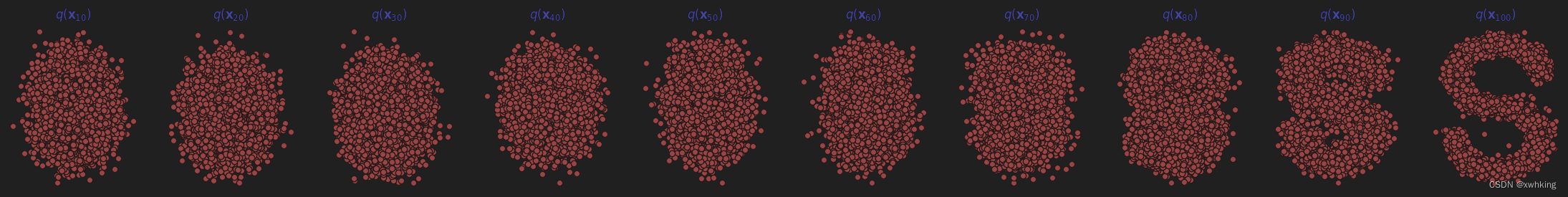
8.开始训练模型，并打印loss以及中间的重构效果

seed = 1234


class EMA():
    """构建一个参数平滑器"""

    def __init__(self, mu=0.01):
        self.mu = mu
        self.shadow = {}

    def register(self, name, val):
        self.shadow[name] = val.clone()

    def __call__(self, name, x):
        assert name in self.shadow
        new_average = self.mu * x + (1.0 - self.mu) * self.shadow[name]
        self.shadow[name] = new_average.clone()
        return new_average


print("training model...")

"""
ema = EMA(0.5)
for name,param in model.named_parameters():
    if param.requires_grad:
        ema.register(name,param.data)
"""

batch_size = 128
dataloader = torch.utils.data.DataLoader(dataset, batch_size=batch_size, shuffle=True)
num_epochs = 4000
plt.rc('text', color='blue')

model = MLPDiffusion(num_steps)  # 输出维度是 2 ，输入还x和step
optimizer = torch.optim.Adam(model.parameters(), lr=1e-3)

for t in range(num_epochs):
    for idx, batch_x in enumerate(dataloader):
        loss = diffusion_loss_fn(model, batch_x, alphas_bar_sqrt, one_minus_alphas_bar_sqrt, num_steps)
        optimizer.zero_grad()
        loss.backward()
        torch.nn.utils.clip_grad_norm_(model.parameters(), 1.)
        optimizer.step()
        # for name,param in model.named_parameters():
        #     if param.requires_grad:
        #         param.data = ema(name,param.data)

    # print loss
    if t % 100 == 0:
        print(loss)
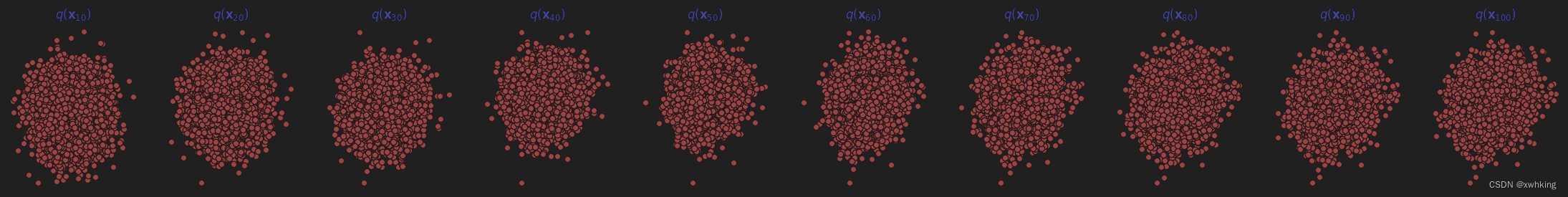
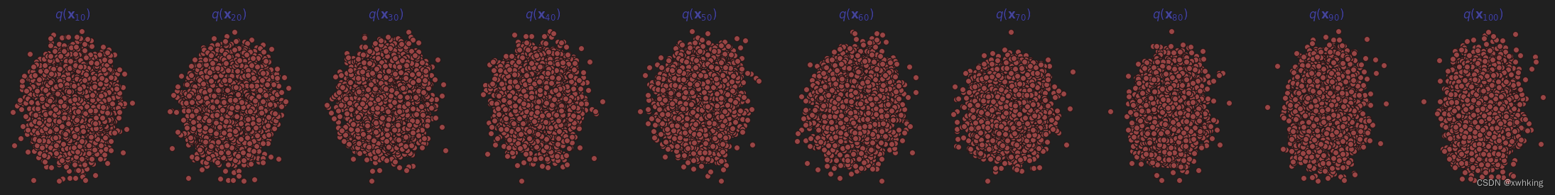
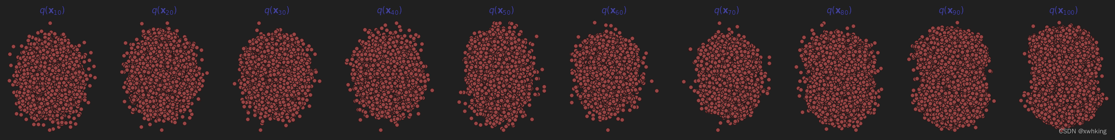
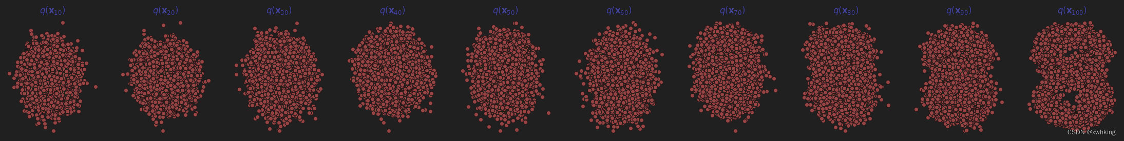
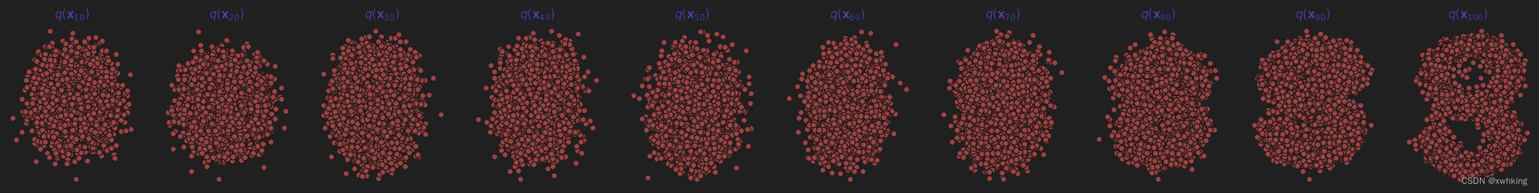
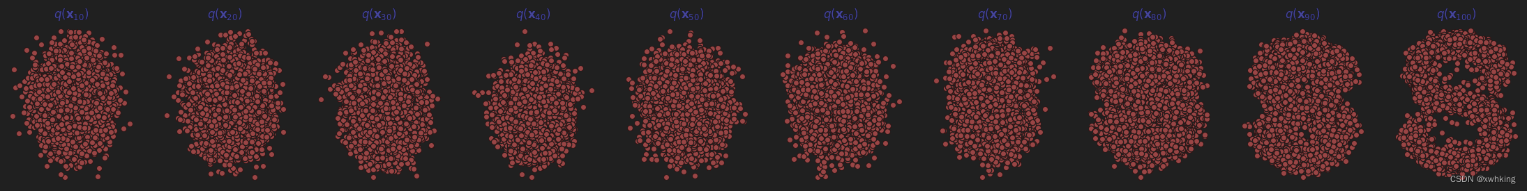
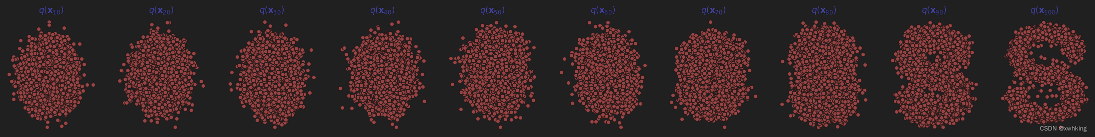
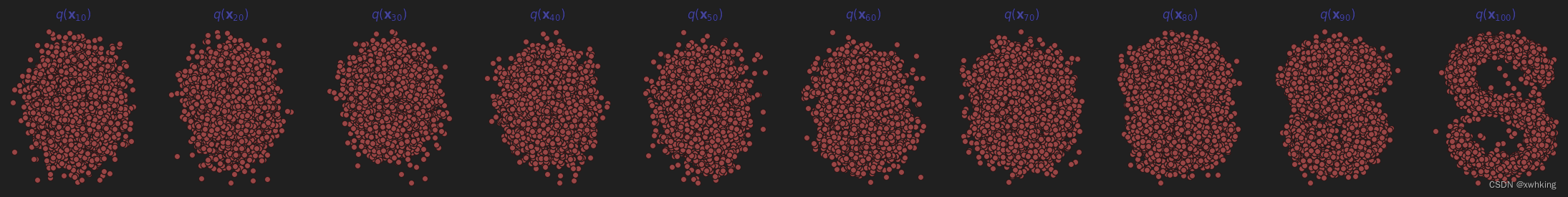
        x_seq = p_sample_loop(model, dataset.shape, num_steps, betas, one_minus_alphas_bar_sqrt)  # 共有 100 个元素
        fig, axs = plt.subplots(1, 10, figsize=(28, 3))
        for i in range(1, 11):
            cur_x = x_seq[i * 10].detach()
            axs[i - 1].scatter(cur_x[:, 0], cur_x[:, 1], color='red', edgecolor='white')
            axs[i - 1].set_axis_off()
            axs[i - 1].set_title('$q(\mathbf{x}_{' + str(i * 10) + '})$')

<>:55: SyntaxWarning: invalid escape sequence '\m'
<>:55: SyntaxWarning: invalid escape sequence '\m'
C:\Users\28374\AppData\Local\Temp\ipykernel_10752\1573120526.py:55: SyntaxWarning: invalid escape sequence '\m'
  axs[i-1].set_title('$q(\mathbf{x}_{' + str(i*10)+'})$')

training model...
tensor(0.8371, grad_fn=<MeanBackward0>)
tensor(0.3398, grad_fn=<MeanBackward0>)
tensor(0.3658, grad_fn=<MeanBackward0>)
tensor(0.2152, grad_fn=<MeanBackward0>)
tensor(0.3706, grad_fn=<MeanBackward0>)
tensor(0.2685, grad_fn=<MeanBackward0>)
tensor(0.4213, grad_fn=<MeanBackward0>)
tensor(0.3830, grad_fn=<MeanBackward0>)
tensor(0.2178, grad_fn=<MeanBackward0>)
tensor(0.1918, grad_fn=<MeanBackward0>)
tensor(0.2116, grad_fn=<MeanBackward0>)
tensor(0.3871, grad_fn=<MeanBackward0>)
tensor(0.3366, grad_fn=<MeanBackward0>)
tensor(0.1989, grad_fn=<MeanBackward0>)
tensor(0.5254, grad_fn=<MeanBackward0>)
tensor(0.2641, grad_fn=<MeanBackward0>)
tensor(0.3108, grad_fn=<MeanBackward0>)
tensor(0.1901, grad_fn=<MeanBackward0>)
tensor(0.5101, grad_fn=<MeanBackward0>)
tensor(0.3037, grad_fn=<MeanBackward0>)
tensor(0.8759, grad_fn=<MeanBackward0>)

C:\Users\28374\AppData\Local\Temp\ipykernel_10752\1573120526.py:50: RuntimeWarning: More than 20 figures have been opened. Figures created through the pyplot interface (`matplotlib.pyplot.figure`) are retained until explicitly closed and may consume too much memory. (To control this warning, see the rcParam `figure.max_open_warning`). Consider using `matplotlib.pyplot.close()`.
  fig,axs = plt.subplots(1,10,figsize=(28,3))

tensor(0.3038, grad_fn=<MeanBackward0>)
tensor(0.4054, grad_fn=<MeanBackward0>)
tensor(0.3833, grad_fn=<MeanBackward0>)
tensor(0.4251, grad_fn=<MeanBackward0>)
tensor(0.3462, grad_fn=<MeanBackward0>)
tensor(0.1814, grad_fn=<MeanBackward0>)
tensor(0.2301, grad_fn=<MeanBackward0>)
tensor(0.4002, grad_fn=<MeanBackward0>)
tensor(0.4273, grad_fn=<MeanBackward0>)
tensor(0.3140, grad_fn=<MeanBackward0>)
tensor(0.3192, grad_fn=<MeanBackward0>)
tensor(0.8542, grad_fn=<MeanBackward0>)
tensor(0.4358, grad_fn=<MeanBackward0>)
tensor(0.2812, grad_fn=<MeanBackward0>)
tensor(0.4819, grad_fn=<MeanBackward0>)
tensor(0.2980, grad_fn=<MeanBackward0>)
tensor(0.4941, grad_fn=<MeanBackward0>)
tensor(0.6179, grad_fn=<MeanBackward0>)
tensor(0.2370, grad_fn=<MeanBackward0>)

<Figure size 2800x300 with 10 Axes>
<Figure size 2800x300 with 10 Axes>
<Figure size 2800x300 with 10 Axes>
<Figure size 2800x300 with 10 Axes>
<Figure size 2800x300 with 10 Axes>
<Figure size 2800x300 with 10 Axes>
<Figure size 2800x300 with 10 Axes>
<Figure size 2800x300 with 10 Axes>
<Figure size 2800x300 with 10 Axes>
<Figure size 2800x300 with 10 Axes>
<Figure size 2800x300 with 10 Axes>
<Figure size 2800x300 with 10 Axes>
<Figure size 2800x300 with 10 Axes>
<Figure size 2800x300 with 10 Axes>
<Figure size 2800x300 with 10 Axes>
<Figure size 2800x300 with 10 Axes>
<Figure size 2800x300 with 10 Axes>
<Figure size 2800x300 with 10 Axes>
<Figure size 2800x300 with 10 Axes>
<Figure size 2800x300 with 10 Axes>
<Figure size 2800x300 with 10 Axes>
<Figure size 2800x300 with 10 Axes>
<Figure size 2800x300 with 10 Axes>
<Figure size 2800x300 with 10 Axes>
<Figure size 2800x300 with 10 Axes>
<Figure size 2800x300 with 10 Axes>
<Figure size 2800x300 with 10 Axes>
<Figure size 2800x300 with 10 Axes>
<Figure size 2800x300 with 10 Axes>
<Figure size 2800x300 with 10 Axes>
<Figure size 2800x300 with 10 Axes>
<Figure size 2800x300 with 10 Axes>
<Figure size 2800x300 with 10 Axes>
<Figure size 2800x300 with 10 Axes>
<Figure size 2800x300 with 10 Axes>
<Figure size 2800x300 with 10 Axes>
<Figure size 2800x300 with 10 Axes>
<Figure size 2800x300 with 10 Axes>
<Figure size 2800x300 with 10 Axes>
<Figure size 2800x300 with 10 Axes>

这里应该会生成 40 张图片，这里只展现能够提现过程的图片了。
在这里插入图片描述

9. 动画演示扩散过程核逆扩散过程

# Generating the forward image sequence 生成前向过程，也就是逐步加噪声
import io
from PIL import Image

imgs = []

for i in range(100):
    plt.clf()
    q_i = q_x(dataset, torch.tensor([i]))
    plt.scatter(q_i[:, 0], q_i[:, 1], color='red', edgecolor='white', s=5)
    plt.axis('off')
    plt.title('step:'+str(i+1))
    img_buf = io.BytesIO()
    plt.savefig(img_buf,format='png')
    img = Image.open(img_buf)
    imgs.append(img)

# Generating the reverse diffusion sequence

reverse = []

for i in range(100):
    plt.clf()
    cur_x = x_seq[i].detach() # 拿到训练末尾阶段生成的 x_seq
    plt.scatter(cur_x[:,0],cur_x[:,1],color='red',edgecolor='white',s=5)
    plt.axis('off')
    plt.title('step:'+str(i+1))
    img_buf = io.BytesIO()
    plt.savefig(img_buf,format='png')
    img = Image.open(img_buf)
    reverse.append(img) 

imgs = imgs + reverse
imgs[0].save("diffusion.gif",format='gif',append_images=imgs,save_all=True,duration=100,loop=1)