数据分析：基于sparcc的co-occurrence网络

介绍

Sparcc是基于16s或metagenomics数据等计算组成数据之间关联关系的算法。通常使用count matrix数据。

安装Sparcc软件

git clone git@github.com:JCSzamosi/SparCC3.git
export PATH=/path/SparCC3:$PATH

which SparCC.py

导入数据

注：使用rarefy抽平的count matrix数据

library(dplyr)
library(tibble)

dat <- read.table("dat_rarefy10000_v2.tsv", header = T)

过滤数据

filter_fun <- function(prof=dat , 
                       tag="dat ", 
                       cutoff=0.005){

  # prof=dat 
  # tag="dat " 
  # cutoff=0.005
  
  dat <- cbind(prof[, 1, drop=F], 
               prof[, -1] %>% summarise(across(everything(), 
                                               function(x){x/sum(x)}))) %>%
    column_to_rownames("OTUID")
  
  #dat.cln <- dat[rowSums(dat) > cutoff, ]
  
  remain <- apply(dat, 1, function(x){
    length(x[x>cutoff])
  }) %>% data.frame() %>%
    setNames("Counts") %>%
    rownames_to_column("OTUID") %>%
    mutate(State=ifelse(Counts>1, "Remain", "Discard")) %>%
    filter(State == "Remain")
  
  # count
  count <- prof %>% filter(OTUID%in%remain$OTUID)
  filename <- paste0("../dataset/Sparcc/", tag, "_rarefy10000_v2_", cutoff, ".tsv")
  write.table(count, file = filename, quote = F, sep = "\t", row.names = F)
  
  # relative abundance
  relative <- dat %>% rownames_to_column("OTUID") %>%
    filter(OTUID%in%remain$OTUID)
  filename <- paste0("../dataset/Sparcc/", tag, "_rarefy10000_v2_", cutoff, "_rb.tsv")
  write.table(relative, file = filename, quote = F, sep = "\t", row.names = F)
}

filter_fun(prof=dat, tag="dat", cutoff=0.005)
filter_fun(prof=dat, tag="dat", cutoff=0.001)

Result：保留过滤后的count matrix和relative abundance matrix两类型矩阵

sparcc analysis

该过程分成两步：1.计算相关系数；2.permutation test计算p值.

iteration 参数使用default -i 20
permutation 参数： 1000次

# Step 1 - Compute correlations
python /data/share/toolkits/SparCC3/SparCC.py sxtr_rarefy10000_v2_0.001.tsv -i 20 --cor_file=sxtr_sparcc.tsv > sxtr_sparcc.log
echo "Step 1 - Compute correlations Ended successfully!"

# Step 2 - Compute bootstraps
python /data/share/toolkits/SparCC3/MakeBootstraps.py sxtr_rarefy10000_v2_0.001.tsv -n 1000 -t bootstrap_#.txt -p pvals/ >> sxtr_sparcc.log
echo "Step 2 - Compute bootstraps Ended successfully!"

# Step 3 - Compute p-values
for n in {0..999}; do /data/share/toolkits/SparCC3/SparCC.py pvals/bootstrap_${n}.txt -i 20 --cor_file=pvals/bootstrap_cor_${n}.txt >> sxtr_sparcc.log; done
python /data/share/toolkits/SparCC3/PseudoPvals.py sxtr_sparcc.tsv pvals/bootstrap_cor_#.txt 1000 -o pvals/pvals.two_sided.txt -t two_sided >> sxtr_sparcc.log
echo "Step 3 - Compute p-values Ended successfully!"

# step 4 - Rename file
mv pvals/pvals.two_sided.txt sxtr_pvals.two_sided.tsv
mv cov_mat_SparCC.out sxtr_cov_mat_SparCC.tsv
echo "step 4 - Rename file Ended successfully!"

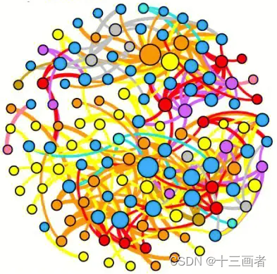
co-occurrence network

网络图要符合以下要求：

保留相互之间显著差异(p < 0.05)OTU;
genus分类学水平表示OTU来源；
OTU间相关性用颜色区分，且线条粗细代表相关系数大小；
OTU点大小表示其丰度大小；
统计网络中正负相关数目；

导入画图数据

library(igraph)
library(psych)

dat_cor <- read.table("dat_cov_mat_SparCC.tsv", header = T, row.names = 1)
dat_pval <- read.table("dat_pvals.two_sided.tsv", header = T, row.names = 1)
dat_rb5 <- read.table("dat_rarefy10000_v2_0.005_rb.tsv", header = T, row.names = 1)
dat_tax <- read.csv("dat_taxonomy.csv")

画图

数据处理
数据可视化
数据存储

cornet_plot <- function(mcor=dat_cor, 
                        mpval=dat_pval, 
                        mrb=dat_rb5, 
                        tax=dat_tax, 
                        type="dat_5"){
  

  # mcor <- dat_cor
  # mpval <- dat_pval
  # mrb <- dat_rb5
  # tax <- dat_tax
  # type="dat_05"
  
  # trim all NA in pvalue < 0.05
  mpval[mpval > 0.05] <- NA
  remain <- apply(mpval, 1, function(x){length(x[!is.na(x)])}) %>% data.frame() %>%
    setNames("counts") %>%
    rownames_to_column("OTUID") %>%
    filter(counts > 0)
  remain_pval <- mpval[as.character(remain$OTUID), as.character(remain$OTUID)]
  
  # remove non significant edges 
  remain_cor <- mcor[as.character(remain$OTUID), as.character(remain$OTUID)]
  for(i in 1:nrow(remain_pval)){
    for(j in 1:ncol(remain_pval)){
      if(is.na(remain_pval[i, j])){
        remain_cor[i, j] <- 0
      }
    }
  }
  
  # OTU relative abundance and taxonomy 
  rb_tax <- mrb %>% rownames_to_column("OTUID") %>%
    filter(OTUID%in%as.character(remain$OTUID)) %>%
    group_by(OTUID) %>%
    rowwise() %>%
    mutate(SumAbundance=mean(c_across(everything()))) %>%
    ungroup() %>%
    inner_join(tax, by="OTUID") %>%
    dplyr::select("OTUID", "SumAbundance", "Genus") %>%
    mutate(Genus=gsub("g__Candidatus", "Ca.", Genus),
           Genus=gsub("_", " ", Genus)) %>%
    mutate(Genus=factor(as.character(Genus)))
  
  # 构建igraph对象
  igraph <- graph.adjacency(as.matrix(remain_cor), mode="undirected", weighted=TRUE, diag=FALSE)
  
  # 去掉孤立点
  bad.vs <- V(igraph)[degree(igraph) == 0]
  igraph <- delete.vertices(igraph, bad.vs)
  
  # 将igraph weight属性赋值到igraph.weight
  igraph.weight <- E(igraph)$weight
  
  # 做图前去掉igraph的weight权重，因为做图时某些layout会受到其影响
  E(igraph)$weight <- NA
  
  
  number_cor <- paste0("postive correlation=", sum(igraph.weight > 0), "\n",
                       "negative correlation=",  sum(igraph.weight < 0))
  
  # set edge color，postive correlation 设定为red, negative correlation设定为blue
  E.color <- igraph.weight
  E.color <- ifelse(E.color > 0, "red", ifelse(E.color < 0, "blue", "grey"))
  E(igraph)$color <- as.character(E.color)
  
  # 可以设定edge的宽 度set edge width，例如将相关系数与edge width关联
  E(igraph)$width <- abs(igraph.weight)
  
  # set vertices size
  igraph.size <- rb_tax %>% filter(OTUID%in%V(igraph)$name) 
  igraph.size.new <- log((igraph.size$SumAbundance) * 1000000)
  V(igraph)$size <- igraph.size.new
  
  # set vertices color
  igraph.col <- rb_tax %>% filter(OTUID%in%V(igraph)$name)
  pointcolor <- c("green","deeppink","deepskyblue","yellow","brown","pink","gray","cyan","peachpuff")
  pr <- levels(igraph.col$Genus)
  pr_color <- pointcolor[1:length(pr)]
  levels(igraph.col$Genus) <- pr_color
  V(igraph)$color <- as.character(igraph.col$Genus)
  
  # 按模块着色
  # fc <- cluster_fast_greedy(igraph, weights=NULL)
  # modularity <- modularity(igraph, membership(fc))
  # comps <- membership(fc)
  # colbar <- rainbow(max(comps))
  # V(igraph)$color <- colbar[comps]
  
  filename <- paste0("../figure/03.Network/", type, "_Sparcc.pdf")
  pdf(file = filename, width = 10, height = 10)
  plot(igraph,
     main="Co-occurrence network",
     layout=layout_in_circle,
     edge.lty=1,
     edge.curved=TRUE,
     margin=c(0,0,0,0))
  legend(x=.8, y=-1, bty = "n",
         legend=pr,
         fill=pr_color, border=NA)
  text(x=.3, y=-1.2, labels=number_cor, cex = 1.5)
  dev.off()
  
  # calculate OTU 
  remain_cor_sum <- apply(remain_cor, 1, function(x){
    res1 <- as.numeric(length(x[x>0]))
    res2 <- as.numeric(length(x[x<0]))
    res <- c(res1, res2)
  }) %>% t() %>% data.frame() %>%
    setNames(c("Negative", "Positive")) %>%
    rownames_to_column("OTUID")
  
  file_cor <- paste0("../figure/03.Network/", type, "_Sparcc_negpos.csv")
  write.csv(remain_cor_sum, file = file_cor, row.names = F)
}

运行画图函数

cornet_plot(mcor=dat_cor, 
            mpval=dat_pval, 
            mrb=dat_rb5, 
            tax=dat_tax, 
            type="dat_5")

在这里插入图片描述

R information

sessionInfo()

R version 4.0.2 (2020-06-22)
Platform: x86_64-w64-mingw32/x64 (64-bit)
Running under: Windows 10 x64 (build 19042)

Matrix products: default

locale:
[1] LC_COLLATE=English_United States.1252  LC_CTYPE=English_United States.1252    LC_MONETARY=English_United States.1252
[4] LC_NUMERIC=C                           LC_TIME=English_United States.1252    
system code page: 936

attached base packages:
[1] stats     graphics  grDevices utils     datasets  methods   base     

other attached packages:
[1] psych_2.0.9  igraph_1.2.5 tibble_3.0.3 dplyr_1.0.2 

loaded via a namespace (and not attached):
 [1] lattice_0.20-41  crayon_1.3.4     grid_4.0.2       R6_2.5.0         nlme_3.1-150     lifecycle_0.2.0  magrittr_1.5    
 [8] pillar_1.4.6     rlang_0.4.7      rstudioapi_0.11  vctrs_0.3.4      generics_0.1.0   ellipsis_0.3.1   tools_4.0.2     
[15] glue_1.4.2       purrr_0.3.4      parallel_4.0.2   xfun_0.19        yaml_2.2.1       compiler_4.0.2   pkgconfig_2.0.3 
[22] mnormt_2.0.2     tmvnsim_1.0-2    knitr_1.30       tidyselect_1.1.0