引言
这个作业的目的是给你们介绍建立,训练和测试神经系统网络模型。您不仅将接触到使用Python包构建神经系统网络从无到有,还有数学方面的反向传播和梯度下降。但在实际情况下,你不一定要实现神经网络从零开始(你们将在以后的实验和作业中看到),这个作业旨在给你们对像TensorFlow和Keras这样的包的底层运行情况有一个初步的了解。在本作业中,您将使用MNIST手写数字数据集来训练一个简单的分类神经网络使用批量学习和评估你的模型。
English(英文):http://t.csdn.cn/p8KTX
Link to this article .pdf file
---------------------------------------------------------------------------------------------------------------------------------
提取码:v6zc
https://pan.baidu.com/s/1_qFbN0Nhc8MNYCHEyTbkLg%C2%A0
实验2:Numpy手写多层神经网络
引言
实验所需文件
文件获取:
文件结构:
概念上的问题
获得模板
获得数据
作业概述:
实验开始之前:
1. 预处理的数据
2. 独热编码
3.核心抽象
4. 网络层
5. 激活函数
6. 填充模型
7、损失函数
8.优化器
9. 精度指标
10. 训练和测试
11. 可视化的结果
CS1470 Students
CS2470 Students
重要的!
参考答案:http://t.csdn.cn/9sdBN
实验所需文件
文件获取:
链接:https://pan.baidu.com/s/1JQnPdOJQXqQ43W74NuYqwg
提取码:2wlg
文件结构:
| - hw2
| - code
| - Beras
| - 8个.py文件用于实现实验要求函数
| - assignment.py
| - preprocess.py
| - visualize.py
| - data
| - mnist
| - 四个数据集文件
概念上的问题
请提交关于Gradescope的概念问题在hw2-mlp概念性下。您必须输入您提交的内容并上传PDF文件。我们建议使用LaTeX。
获得模板
Github Classroom Link with Stencil Code!
Guide on GitHub and GitHub Classroom
获得数据
可使用download.sh下载数据。方法可以运行bash脚本命令。/script_name.sh(例如:bash ./download.sh)。这与HW1类似。使用除去所提供的模板代码,但除非指定,否则不要更改模板。这样做可能会导致与自动分级程序不兼容。不要更改任何方法和变量!这个作业需要NumPy和Matplotlib。你应该已经从HW1得到这个了。
作业概述:
在这个作业中,你将构建一个Keras模仿,Beras(哈哈有趣的名字),并将制定一个模仿Tensorflow/Keras API的顺序模型规范。Python与本作业相关的笔记本是为了让您探索一个示例实现这样你就可以自己动手了!笔记本上没有什么待办事项需要你去做;相反,测试是通过运行assign .py的主要方法来完成的。我们的模板提供了一个模型类,其中包含您需要使用的几个方法和超参数你的网络。
实验开始之前:
这份家庭作业在发布两周后到期。实验室1-3提供了很好的练习这个任务,所以如果你卡住了,你可以等他们一会儿。具体地说:
☆ -实现可调用/可扩散组件:实现此目标所需的技能可以通过实验室1找到。这包括对数学的精通符号、矩阵运算以及调用和梯度方法背后的逻辑。
☆ -实现优化器:您可以通过以下方法实现BasicOptimizer类按照实验室1中gradient - descent方法的逻辑。其他的优化(例如Adam, RMSProp)将在实验室2:优化器中讨论。
☆ -使用batch_step和GradientTape:您可以了解如何使用它们来训练您的基于赋值指令和这些指令的实现进行建模。与也就是说,他们确实模仿了Keras API。你将在实验3:介绍中了解所有这些Tensorflow。如果你的实验在截止日期之后,应该没问题;浏览一下与实验室相关的补充笔记本。你可以先做你能做的,然后在学习更多关于深度的知识时再添加。学习并意识到你在课堂上学到的概念实际上可以在这里使用!不要气馁,试着玩得开心点!
路线图:在这个作业中,我们会带你走过神经网络训练的流程,包括模型类的结构和您必须填写的方法。
1. 预处理的数据
在训练网络之前,需要清理数据。这包括检索、更改数据并将其格式化为网络的输入。对于这个任务,您将处理MNIST数据集。它可以通过下载.sh脚本,但它也链接在这里(忽略它所说的hw1;我们使用这个这次是hw2的数据集!)。原始数据源在这里。您应该只使用训练数据训练网络,然后测试网络测试数据的准确性。你的程序应该在测试中打印出它的准确性数据集完成后。
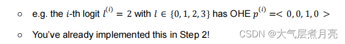
2. 独热编码
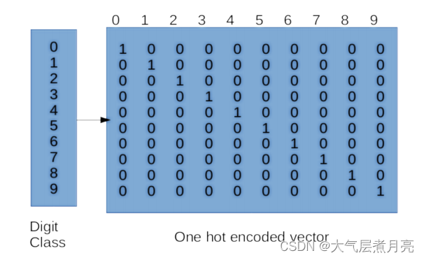
在训练或测试模型之前,您需要对类标签进行“one-hot”编码因此,该模型可以优化到预测任何期望的类。注意,类标签本身就是简单的类别,在数字上没有任何意义。在如果没有单热编码,您的模型可能会学习之间的一些自然排序基于标签的不同类标签(标签是任意的)。例如,假设有一个数据点a对应标签“2”和一个数据点B对应于标签' 7 '。我们不想让模型知道B比a的权重高,因为从数字上讲,7 > 2。要一次性编码你的类标签,你需要必须转换你的一维标签向量吗到大小为num_classes的向量中(其中中的类的总数你的数据集)。对于MNIST数据集,它是这样的类似于右边的矩阵:
您必须在Beras/onehot.py中填写以下方法:
●fit(): [TODO] 在这个函数中,你需要在Data(将其存储在self.uniq中)并创建一个以标签作为键的字典和它们对应的一个热编码作为值。提示:你可能想这么做查看np.eye()以获得单热编码。最终,您将存储它在self.uniq2oh字典。
●forward(): 在这个函数中,我们传递一个向量,包含对象中所有实际的标签训练集并调用fit()来用unique填充uniq2oh字典标签及其对应的one-hot编码,然后使用它返回一个针对训练集中每个标签的单热编码标签数组。
这个函数已经为您填好了!
●inverse(): 在函数中,我们将one-hot编码反转为实际编码标签。
这已经为你做过了。
例如,如果我们有标签X和Y,其单热编码为[1,0]和[0,1],我们将
{X: [1,0], Y:[0,1]}。如上图所示,
对于MNIST,你将有10个标签,所以你的字典应该有10个条目!
您可能会注意到,有些类继承自Callable或Diffable。更多关于这
在下一节!
import numpy as np

from .core import Callable


class OneHotEncoder(Callable):
    """
    One-Hot Encodes labels. First takes in a candidate set to figure out what elements it
    needs to consider, and then one-hot encodes subsequent input datasets in the
    forward pass.

    SIMPLIFICATIONS:
     - Implementation assumes that entries are individual elements.
     - Forward will call fit if it hasn't been done yet; most implementations will just error.
     - keras does not have OneHotEncoder; has LabelEncoder, CategoricalEncoder, and to_categorical()
    """

    def fit(self, data):
        """
        Fits the one-hot encoder to a candidate dataset. Said dataset should contain
        all encounterable elements.

        :param data: 1D array containing labels.
            For example, data = [0, 1, 3, 3, 1, 9, ...]
        """
        ## TODO: Fetch all the unique labels and create a dictionary with
        ## the unique labels as keys and their one hot encodings as values
        ## HINT: look up np.eye() and see if you can utilize it!

        ## HINT: Wouldn't it be nice if we just gave you the implementation somewhere...

        self.uniq = None  # all the unique labels from `data`
        self.uniq2oh = None  # a lookup dictionary with labels and corresponding encodings

    def forward(self, data):
        if not hasattr(self, "uniq2oh"):
            self.fit(data)
        return np.array([self.uniq2oh[x] for x in data])

    def inverse(self, data):
        assert hasattr(self, "uniq"), \
            "forward() or fit() must be called before attempting to invert"
        return np.array([self.uniq[x == 1][0] for x in data])
3.核心抽象
考虑以下模块的抽象类。一定要玩一下与此相关的Python笔记本作业,可以很好地掌握核心在Beras/core.py中为您定义的抽象模块!笔记本是探索性的(它不是必需的,所有的代码都给出了),并将为您提供许多深入理解和使用这些类抽象!注意以下模块与Tensorflow/Keras API非常相似。
可调用的:具有定义良好的前向函数的函数。这些是你需要的实现:
● CategoricalAccuracy (./metrics.py):计算预测的精度概率与基本事实标签列表的对比。由于精度没有优化,没有必要计算它的梯度。此外,类别准确性是分段不连续,所以梯度在技术上是0或无定义的。
● OneHotEncoder (./onehot.py):你可以将一个类实例one-hot编码到一个优化概率分布,分类为离散的选项:
可分化的:也可分化的可调用对象。我们可以把这些用在我们的生产线上并通过它们进行优化!因此,大多数这些类都是为在您的神经系统中使用而创建的网络层。这些是你需要实现的:
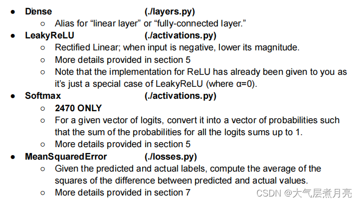
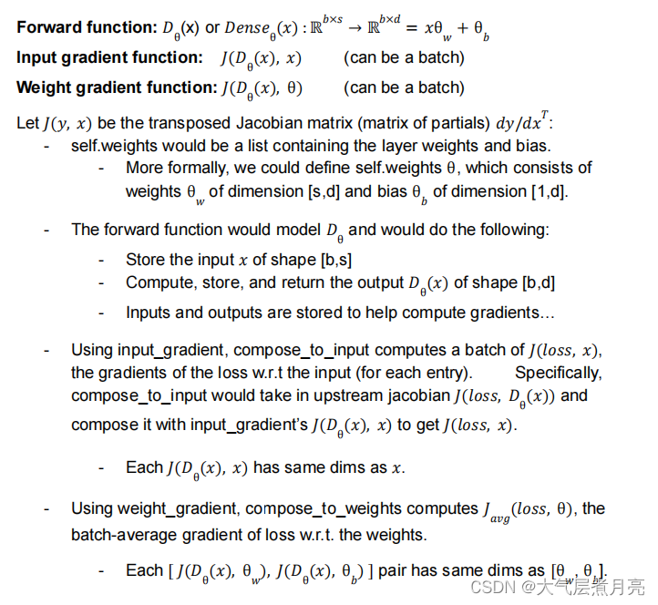
示例:考虑一个致密层实例。让s表示输入大小(源),d表示输出大小(目标),b表示批处理大小。然后:
GradientTape:这个类的功能完全类似于tf.GradientTape()(参见实验3)。你可以把GradientTape看作记录器。每次操作在梯度磁带的作用域,它记录了发生的操作。然后,在
Backprop,我们可以计算所有操作的梯度。这允许我们对任意中间步骤求最终输出的微分。当操作计算在GradientTape的范围之外,他们不会被记录,所以你的代码会没有它们的记录,不能计算梯度。您可以查看这是如何在核心实现的!当然,Tensorflow的梯度磁带的实现要复杂得多,需要构建一个图表。
●[TODO]实现梯度方法,它返回一个梯度列表,对应于网络中可训练的权重列表。代码中的详细信息。
from abc import ABC, abstractmethod  # # For abstract method support
from typing import Tuple

import numpy as np


## DO NOT MODIFY THIS CLASS
class Callable(ABC):
    """
    Callable Sub-classes:
     - CategoricalAccuracy (./metrics.py)       - TODO
     - OneHotEncoder       (./preprocess.py)    - TODO
     - Diffable            (.)                  - DONE
    """

    def __call__(self, *args, **kwargs) -> np.array:
        """Lets `self()` and `self.forward()` be the same"""
        return self.forward(*args, **kwargs)

    @abstractmethod
    def forward(self, *args, **kwargs) -> np.array:
        """Pass inputs through function. Can store inputs and outputs as instance variables"""
        pass


## DO NOT MODIFY THIS CLASS
class Diffable(Callable):
    """
    Diffable Sub-classes:
     - Dense            (./layers.py)           - TODO
     - LeakyReLU, ReLU  (./activations.py)      - TODO
     - Softmax          (./activations.py)      - TODO
     - MeanSquaredError (./losses.py)           - TODO
    """

    """Stores whether the operation being used is inside a gradient tape scope"""
    gradient_tape = None  ## All-instance-shared variable

    def __init__(self):
        """Is the layer trainable"""
        super().__init__()
        self.trainable = True  ## self-only instance variable

    def __call__(self, *args, **kwargs) -> np.array:
        """
        If there is a gradient tape scope in effect, perform AND RECORD the operation.
        Otherwise... just perform the operation and don't let the gradient tape know.
        """
        if Diffable.gradient_tape is not None:
            Diffable.gradient_tape.operations += [self]
        return self.forward(*args, **kwargs)

    @abstractmethod
    def input_gradients(self: np.array) -> np.array:
        """Returns gradient for input (this part gets specified for all diffables)"""
        pass

    def weight_gradients(self: np.array) -> Tuple[np.array, np.array]:
        """Returns gradient for weights (this part gets specified for SOME diffables)"""
        return ()

    def compose_to_input(self, J: np.array) -> np.array:
        """
        Compose the inputted cumulative jacobian with the input jacobian for the layer.
        Implemented with batch-level vectorization.

        Requires `input_gradients` to provide either batched or overall jacobian.
        Assumes input/cumulative jacobians are matrix multiplied
        """
        #  print(f"Composing to input in {self.__class__.__name__}")
        ig = self.input_gradients()
        batch_size = J.shape[0]
        n_out, n_in = ig.shape[-2:]
        j_new = np.zeros((batch_size, n_out), dtype=ig.dtype)
        for b in range(batch_size):
            ig_b = ig[b] if len(ig.shape) == 3 else ig
            j_new[b] = ig_b @ J[b]
        return j_new

    def compose_to_weight(self, J: np.array) -> list:
        """
        Compose the inputted cumulative jacobian with the weight jacobian for the layer.
        Implemented with batch-level vectorization.

        Requires `weight_gradients` to provide either batched or overall jacobian.
        Assumes weight/cumulative jacobians are element-wise multiplied (w/ broadcasting)
        and the resulting per-batch statistics are averaged together for avg per-param gradient.
        """
        # print(f'Composing to weight in {self.__class__.__name__}')
        assert hasattr(
            self, "weights"
        ), f"Layer {self.__class__.__name__} cannot compose along weight path"
        J_out = []
        ## For every weight/weight-gradient pair...
        for w, wg in zip(self.weights, self.weight_gradients()):
            batch_size = J.shape[0]
            ## Make a cumulative jacobian which will contribute to the final jacobian
            j_new = np.zeros((batch_size, *w.shape), dtype=wg.dtype)
            ## For every element in the batch (for a single batch-level gradient updates)
            for b in range(batch_size):
                ## If the weight gradient is a batch of transform matrices, get the right entry.
                ## Allows gradient methods to give either batched or non-batched matrices
                wg_b = wg[b] if len(wg.shape) == 3 else wg
                ## Update the batch's Jacobian update contribution
                j_new[b] = wg_b * J[b]
            ## The final jacobian for this weight is the average gradient update for the batch
            J_out += [np.mean(j_new, axis=0)]
        ## After new jacobian is computed for each weight set, return the list of gradient updatates
        return J_out


class GradientTape:

    def __init__(self):
        ## Log of operations that were performed inside tape scope
        self.operations = []

    def __enter__(self):
        # When tape scope is entered, let Diffable start recording to self.operation
        Diffable.gradient_tape = self
        return self

    def __exit__(self, exc_type, exc_val, exc_tb):
        # When tape scope is exited, stop letting Diffable record
        Diffable.gradient_tape = None

    def gradient(self) -> list:
        """Get the gradient from first to last recorded operation"""
        ## TODO:
        ##
        ##  Compute weight gradients for all operations.
        ##  If the model has trainable weights [w1, b1, w2, b2] and ends at a loss L.
        ##  the model should return: [dL/dw1, dL/db1, dL/dw2, dL/db2]
        ##
        ##  Recall that self.operations is populated by Diffable class instances...
        ##
        ##  Start from the last operation and compute jacobian w.r.t input.
        ##  Continue to propagate the cumulative jacobian through the layer inputs
        ##  until all operations have been differentiated through.
        ##
        ##  If an operation that has weights is encountered along the way,
        ##  compute the weight gradients and add them to the return list.
        ##  Remember to check if the layer is trainable before doing this though...

        grads = []
        return grads
4. 网络层
在本文中,您将实现在您的在Beras/layers.py中的顺序模型。你必须填写下列方法:
● forward() : [TODO] 实现向前传递和返回输出。
● weight_gradients() : [TODO] 计算关于的梯度权重和偏差。这将用于优化图层。
● input_gradients() : [TODO] 计算关于的梯度层的输入。这将用于将渐变传播到前面的层。
● _initialize_weight() : [TODO] 初始化致密层的权重值默认情况下,将所有权重初始化为零(顺便说一下,这通常是个坏主意)。你也需要允许更复杂的选项(当初始化式为设置为normal, xavier和kaiing)。遵循Keras的数学假设!
〇 Normal:不言自明,单位正态分布。
〇 Xavier Normal:基于keras.GlorotNormal。
〇 Kaiing He Normal:基于Keras.HeNormal。
在实现这些时,你可能会发现np.random.normal很有帮助。的行动计划说明为什么这些不同的初始化方法是必要的,但是欲了解更多细节,请查看这个网站!请随意添加更多初始化器选项!
import numpy as np

from .core import Diffable


class Dense(Diffable):

    # https://towardsdatascience.com/weight-initialization-in-neural-networks-a-journey-from-the-basics-to-kaiming-954fb9b47c79

    def __init__(self, input_size, output_size, initializer="kaiming"):
        super().__init__()
        self.w, self.b = self.__class__._initialize_weight(
            initializer, input_size, output_size
        )
        self.weights = [self.w, self.b]
        self.inputs  = None
        self.outputs = None

    def forward(self, inputs):
        """Forward pass for a dense layer! Refer to lecture slides for how this is computed."""
        self.inputs = inputs

        # TODO: implement the forward pass and return the outputs
        self.outputs = None
        return self.outputs

    def weight_gradients(self):
        """Calculating the gradients wrt weights and biases!"""
        # TODO: Implement calculation of gradients
        wgrads = None
        bgrads = None
        return wgrads, bgrads

    def input_gradients(self):
        """Calculating the gradients wrt inputs!"""
        # TODO: Implement calculation of gradients
        return None

    @staticmethod
    def _initialize_weight(initializer, input_size, output_size):
        """
        Initializes the values of the weights and biases. The bias weights should always start at zero.
        However, the weights should follow the given distribution defined by the initializer parameter
        (zero, normal, xavier, or kaiming). You can do this with an if statement
        cycling through each option!

        Details on each weight initialization option:
            - Zero: Weights and biases contain only 0's. Generally a bad idea since the gradient update
            will be the same for each weight so all weights will have the same values.
            - Normal: Weights are initialized according to a normal distribution.
            - Xavier: Goal is to initialize the weights so that the variance of the activations are the
            same across every layer. This helps to prevent exploding or vanishing gradients. Typically
            works better for layers with tanh or sigmoid activation.
            - Kaiming: Similar purpose as Xavier initialization. Typically works better for layers
            with ReLU activation.
        """

        initializer = initializer.lower()
        assert initializer in (
            "zero",
            "normal",
            "xavier",
            "kaiming",
        ), f"Unknown dense weight initialization strategy '{initializer}' requested"
        io_size = (input_size, output_size)

        # TODO: Implement default assumption: zero-init for weights and bias

        # TODO: Implement remaining options (normal, xavier, kaiming initializations). Note that
        # strings must be exactly as written in the assert above

        return None, None
5. 激活函数
在这次作业中,你将实现两个主要的激活功能,即:Beras/activation .py中的LeakyReLU和Softmax。因为ReLU是一个特例的LeakyReLU,我们已经提供了它的代码。
● LeakyReLU ()
〇 forward() : [TODO]给定输入x,计算并返回LeakyReLU(x)。
〇 input_gradients() : [TODO]计算并返回与通过对LeakyReLU求导得到输入。
● Softmax():(2470 ONLY)
forward(): [TODO]给定输入x,计算并返回Softmax(x)。确保使用的是稳定的softmax,即减去所有项的最大值防止溢出/undvim erflow问题。
〇 input_gradients(): [TODO] Softmax()的部分w.r.t输入。
import numpy as np

from .core import Diffable


class LeakyReLU(Diffable):
    def __init__(self, alpha=0.3):
        super().__init__()
        self.alpha = alpha
        self.inputs = None
        self.outputs = None

    def forward(self, inputs):
        # TODO: Given an input array `x`, compute LeakyReLU(x)
        self.inputs = inputs
        # Your code here:
        self.outputs = None
        return self.outputs

    def input_gradients(self):
        # TODO: Compute and return the gradients
        return 0

    def compose_to_input(self, J):
        # TODO: Maybe you'll want to override the default?
        return super().compose_to_input(J)


class ReLU(LeakyReLU):
    def __init__(self):
        super().__init__(alpha=0)


class Softmax(Diffable):
    def __init__(self):
        super().__init__()
        self.inputs = None
        self.outputs = None

    def forward(self, inputs):
        """Softmax forward pass!"""
        # TODO: Implement
        # HINT: Use stable softmax, which subtracts maximum from
        # all entries to prevent overflow/underflow issues
        self.inputs = inputs
        # Your code here:
        self.outputs = None
        return self.outputs

    def input_gradients(self):
        """Softmax backprop!"""
        # TODO: Compute and return the gradients
        return 0
6. 填充模型
有了这些抽象概念,让我们为顺序深度学习创建一个序列模型。你可以在assignment.py中找到SequentialModel类初始化你的神经网络的层,参数(权重和偏差),和超参数(优化器、损失函数、学习率、精度函数等)。的SequentialModel类继承自Beras/model.py,在那里您可以找到许多有用的方法。这还将包含适合您的数据和模型的函数评估你的模型的性能:
● compile() : 初始化模型优化器,损失函数和精度函数,它们作为参数输入,供SequentialModel实例使用。
● fit() : 训练模型将输入和输出关联起来。重复训练每个时代,数据是基于参数的批处理。它还计算Batch_metrics、epoch_metrics和聚合的agg_metrics可以用来跟踪模型的训练进度。
● evaluate() : [TODO] 评估最终模型的性能使用测试阶段中提到的指标。它几乎和符合()函数;想想培训和测试之间会发生什么变化)。
● call() : [TODO] 提示:调用顺序模型意味着什么?还记得顺序模型是一堆层,每一层只有一个输入向量和一个输出向量。你可以在在assignment.py中的SequentialModel类。
● batch_step() : [TODO] 您将看到fit()为每一个都调用了这个函数批处理。您将首先计算输入批处理的模型预测。在训练阶段,你需要计算梯度和更新你的权重根据您正在使用的优化器。对于训练过程中的反向传播,你将使用GradientTape从核心抽象(core.py)来记录操作和中间值。然后您将使用模型的优化器来将梯度应用到模型的可训练变量上。最后,计算和
返回该批次的损耗和精度。你可以在在assignment.py中的SequentialModel类。
我们鼓励你去看看keras。在介绍笔记本中的SequentialModel(在探索一个可能的模块化实现:TensorFlow/Keras)和参考来到实验室3,感受一下我们如何在深度学习中使用梯度磁带.
from abc import ABC, abstractmethod
from collections import defaultdict

import numpy as np

from .core import Diffable


def print_stats(stat_dict, b=None, b_num=None, e=None, avg=False):
    """
    Given a dictionary of names statistics and batch/epoch info,
    print them in an appealing manner. If avg, display stat averages.
    """
    title_str = " - "
    if e is not None:
        title_str += f"Epoch {e+1:2}: "
    if b is not None:
        title_str += f"Batch {b+1:3}"
        if b_num is not None:
            title_str += f"/{b_num}"
    if avg:
        title_str += f"Average Stats"
    print(f"\r{title_str} : ", end="")
    op = np.mean if avg else lambda x: x
    print({k: np.round(op(v), 4) for k, v in stat_dict.items()}, end="")
    print("   ", end="" if not avg else "\n")


def update_metric_dict(super_dict, sub_dict):
    """
    Appends the average of the sub_dict metrics to the super_dict's metric list
    """
    for k, v in sub_dict.items():
        super_dict[k] += [np.mean(v)]


class Model(ABC):

    ###############################################################################################
    ## BEGIN GIVEN

    def __init__(self, layers):
        """
        Initialize all trainable parameters and take layers as inputs
        """
        # Initialize all trainable parameters
        assert all([issubclass(layer.__class__, Diffable) for layer in layers])
        self.layers = layers
        self.trainable_variables = []
        for layer in layers:
            if hasattr(layer, "weights") and layer.trainable:
                for weight in layer.weights:
                    self.trainable_variables += [weight]

    def compile(self, optimizer, loss_fn, acc_fn):
        """
        "Compile" the model by taking in the optimizers, loss, and accuracy functions.
        In more optimized DL implementations, this will have more involved processes
        that make the components extremely efficient but very inflexible.
        """
        self.optimizer = optimizer
        self.compiled_loss = loss_fn
        self.compiled_acc = acc_fn

    def fit(self, x, y, epochs, batch_size):
        """
        Trains the model by iterating over the input dataset and feeding input batches
        into the batch_step method with training. At the end, the metrics are returned.
        """
        agg_metrics = defaultdict(lambda: [])
        batch_num = x.shape[0] // batch_size
        for e in range(epochs):
            epoch_metrics = defaultdict(lambda: [])
            for b, b1 in enumerate(range(batch_size, x.shape[0] + 1, batch_size)):
                b0 = b1 - batch_size
                batch_metrics = self.batch_step(x[b0:b1], y[b0:b1], training=True)
                update_metric_dict(epoch_metrics, batch_metrics)
                print_stats(batch_metrics, b, batch_num, e)
            update_metric_dict(agg_metrics, epoch_metrics)
            print_stats(epoch_metrics, e=e, avg=True)
        return agg_metrics

    def evaluate(self, x, y, batch_size):
        """
        X is the dataset inputs, Y is the dataset labels.
        Evaluates the model by iterating over the input dataset in batches and feeding input batches
        into the batch_step method. At the end, the metrics are returned. Should be called on
        the testing set to evaluate accuracy of the model using the metrics output from the fit method.

        NOTE: This method is almost identical to fit (think about how training and testing differ --
        the core logic should be the same)
        """
        # TODO: Implement evaluate similarly to fit.
        agg_metrics = defaultdict(lambda: [])
        return agg_metrics

    @abstractmethod
    def call(self, inputs):
        """You will implement this in the SequentialModel class in assignment.py"""
        return

    @abstractmethod
    def batch_step(self, x, y, training=True):
        """You will implement this in the SequentialModel class in assignment.py"""
        return
7、损失函数
这是模型训练中最关键的方面之一。在这次作业中,我们会实现MSE或均方误差损失函数。你可以找到损失函数在Beras/ losses.py。
● forward() : [TODO] 编写一个计算并返回平均值的函数给出预测和实际标签的平方误差。
提示:什么是MSE?在给出预测和实际标签的情况下,均方误差是预测值与实际值之间的差异。
● input_gradients() : [TODO] 计算并返回梯度。使用用微分法推导出这些梯度的公式。
import numpy as np

from .core import Diffable


class MeanSquaredError(Diffable):
    def __init__(self):
        super().__init__()
        self.y_pred  = None
        self.y_true  = None
        self.outputs = None

    def forward(self, y_pred, y_true):
        """Mean squared error forward pass!"""
        # TODO: Compute and return the MSE given predicted and actual labels
        self.y_pred = y_pred
        self.y_true = y_true

        # Your code here:
        self.outputs = None
        return None

    # https://medium.com/analytics-vidhya/derivative-of-log-loss-function-for-logistic-regression-9b832f025c2d
    def input_gradients(self):
        """Mean squared error backpropagation!"""
        # TODO: Compute and return the gradients
        return None


def clip_0_1(x, eps=1e-8):
    return np.clip(x, eps, 1-eps)

class CategoricalCrossentropy(Diffable):
    """
    GIVEN. Feel free to use categorical cross entropy as your loss function for your final model.

    https://medium.com/analytics-vidhya/derivative-of-log-loss-function-for-logistic-regression-9b832f025c2d
    """

    def __init__(self):
        super().__init__()
        self.truths  = None
        self.inputs  = None
        self.outputs = None

    def forward(self, inputs, truths):
        """Categorical cross entropy forward pass!"""
        # print(truth.shape, inputs.shape)
        ll_right = truths * np.log(clip_0_1(inputs))
        ll_wrong = (1 - truths) * np.log(clip_0_1(1 - inputs))
        nll_total = -np.mean(ll_right + ll_wrong, axis=-1)

        self.inputs = inputs
        self.truths = truths
        self.outputs = np.mean(nll_total, axis=0)
        return self.outputs

    def input_gradients(self):
        """Categorical cross entropy backpropagation!"""
        bn, n = self.inputs.shape
        grad = np.zeros(shape=(bn, n), dtype=self.inputs.dtype)
        for b in range(bn):
            inp = self.inputs[b]
            tru = self.truths[b]
            grad[b] = inp - tru
            grad[b] /= clip_0_1(inp - inp ** 2)
            grad[b] /= inp.shape[-1]
        return grad
8.优化器
在Beras/optimizer .py文件中,确保为每个不同类型的优化器。实验二应该能帮上忙,祝你好运!
● BasicOptimizer : [TODO] 一个简单的优化器策略,如实验1所示。
● RMSProp : [TODO] 误差传播的均方根。
● Adam : [TODO] 一个常见的基于自适应运动估计的优化器。
from collections import defaultdict
import numpy as np

## HINT: Lab 2 might be helpful...

class BasicOptimizer:
    def __init__(self, learning_rate):
        self.learning_rate = learning_rate

    def apply_gradients(self, weights, grads):
        # TODO: Update the weights using basic stochastic gradient descent
        return


class RMSProp:
    def __init__(self, learning_rate, beta=0.9, epsilon=1e-6):
        self.learning_rate = learning_rate

        self.beta = beta
        self.epsilon = epsilon

        self.v = defaultdict(lambda: 0)

    def apply_gradients(self, weights, grads):
        # TODO: Implement RMSProp optimization
        # Refer to the lab on Optimizers for a better understanding!
        return


class Adam:
    def __init__(
        self, learning_rate, beta_1=0.9, beta_2=0.999, epsilon=1e-7, amsgrad=False
    ):
        self.amsgrad = amsgrad

        self.learning_rate = learning_rate
        self.beta_1 = beta_1
        self.beta_2 = beta_2
        self.epsilon = epsilon

        self.m = defaultdict(lambda: 0)  # First moment zero vector
        self.v = defaultdict(lambda: 0)  # Second moment zero vector.
        # Expected value of first moment vector
        self.m_hat = defaultdict(lambda: 0)
        # Expected value of second moment vector
        self.v_hat = defaultdict(lambda: 0)
        self.t = 0  # Time counter

    def apply_gradients(self, weights, grads):
        # TODO: Implement Adam optimization
        # Refer to the lab on Optimizers for a better understanding!
        return
9. 精度指标
最后,为了评估模型的性能,您需要使用适当的精度指标。在这项作业中,你将在Beras/ metrics.py实现评估分类的准确性:
● forward() : [TODO] 返回模型的分类精度预测概率和真标签。你应该返回的比例预测标签等于真实标签,其中图像的预测标签为与最高概率对应的标签。参考网络或讲座幻灯片的分类精度数学!
import numpy as np

from .core import Callable


class CategoricalAccuracy(Callable):
    def forward(self, probs, labels):
        """Categorical accuracy forward pass!"""
        super().__init__()
        # TODO: Compute and return the categorical accuracy of your model given the output probabilities and true labels
        return None
10. 训练和测试
最后,使用上述所有原语,您需要在其中构建两个模型assignment.py:
● get_simple_model()中的一个简单模型,最多只有一个扩散层(例如:density - ./layers.py)和一个激活函数(在/ activation.py)。虽然可以这样做,但默认情况下为您提供了这个选项。如果你愿意,可以改一下。自动评分器将评估原始的一个!
● get_advanced_model()中稍微复杂一点的模型,有两个或更多扩散层和两个或两个以上的激活函数。我们推荐使用Adam该模型的优化器具有相当低的学习率。

对于您使用的任何超参数(层大小,学习率,历元大小,批处理大小,等),请硬编码这些值在get_simple_model()和get_advanced_model()函数。不要将它们存储在主处理程序下。一旦一切都实现了,就可以使用python3 assignment.py来运行你的建模,看看损失/精度!
from types import SimpleNamespace

import Beras
import numpy as np


class SequentialModel(Beras.Model):
    """
    Implemented in Beras/model.py

    def __init__(self, layers):
    def compile(self, optimizer, loss_fn, acc_fn):
    def fit(self, x, y, epochs, batch_size):
    def evaluate(self, x, y, batch_size):           ## <- TODO
    """

    def call(self, inputs):
        """
        Forward pass in sequential model. It's helpful to note that layers are initialized in Beras.Model, and
        you can refer to them with self.layers. You can call a layer by doing var = layer(input).
        """
        # TODO: The call function!
        return None

    def batch_step(self, x, y, training=True):
        """
        Computes loss and accuracy for a batch. This step consists of both a forward and backward pass.
        If training=false, don't apply gradients to update the model!
        Most of this method (forward, loss, applying gradients)
        will take place within the scope of Beras.GradientTape()
        """
        # TODO: Compute loss and accuracy for a batch.
        # If training, then also update the gradients according to the optimizer
        return {"loss": None, "acc": None}


def get_simple_model_components():
    """
    Returns a simple single-layer model.
    """
    ## DO NOT CHANGE IN FINAL SUBMISSION

    from Beras.activations import Softmax
    from Beras.layers import Dense
    from Beras.losses import MeanSquaredError
    from Beras.metrics import CategoricalAccuracy
    from Beras.optimizers import BasicOptimizer

    # TODO: create a model and compile it with layers and functions of your choice
    model = SequentialModel([Dense(784, 10), Softmax()])
    model.compile(
        optimizer=BasicOptimizer(0.02),
        loss_fn=MeanSquaredError(),
        acc_fn=CategoricalAccuracy(),
    )
    return SimpleNamespace(model=model, epochs=10, batch_size=100)


def get_advanced_model_components():
    """
    Returns a multi-layered model with more involved components.
    """
    # TODO: create/compile a model with layers and functions of your choice.
    # model = SequentialModel()

    return SimpleNamespace(model=None, epochs=None, batch_size=None)


if __name__ == "__main__":
    """
    Read in MNIST data and initialize/train/test your model.
    """
    from Beras.onehot import OneHotEncoder
    import preprocess

    ## Read in MNIST data,
    train_inputs, train_labels = preprocess.get_data_MNIST("train", "../data")
    test_inputs,  test_labels  = preprocess.get_data_MNIST("test",  "../data")

    ## TODO: Use the OneHotEncoder class to one hot encode the labels
    ohe = lambda x: 0  ## placeholder function: returns zero for a given input

    ## Get your model to train and test
    simple = False
    args = get_simple_model_components() if simple else get_advanced_model_components()
    model = args.model

    ## REMINDER: Threshold of accuracy:
    ##  1470: >85% on testing accuracy from get_simple_model_components
    ##  2470: >95% on testing accuracy from get_advanced_model_components

    # TODO: Fit your model to the training input and the one hot encoded labels
    # Remember to pass all the arguments that SequentialModel.fit() requires
    # such as number of epochs and the batch size
    train_agg_metrics = model.fit(
        train_inputs,
        ohe(train_labels),
        epochs     = args.epochs,
        batch_size = args.batch_size
    )

    ## Feel free to use the visualize_metrics function to view your accuracy and loss.
    ## The final accuracy returned during evaluation must be > 80%.

    # from visualize import visualize_images, visualize_metrics
    # visualize_metrics(train_agg_metrics["loss"], train_agg_metrics["acc"])
    # visualize_images(model, train_inputs, ohe(train_labels))

    ## TODO: Evaluate your model using your testing inputs and one hot encoded labels.
    ## This is the number you will be using!
    test_agg_metrics = model.evaluate(test_inputs, ohe(test_labels), batch_size=100)
    print('Testing Performance:', test_agg_metrics)
11. 可视化的结果
我们为您提供了visualize_metrics方法来可视化您的损失和每次使用matplotlib后,精确度都会发生变化。不要编辑此函数。在存储了损失和精度之后,应该在主方法中调用这个函数数组中的每个批处理,将传递给此函数。这应该是一条线横轴是第i批,纵轴是批量损失/精度值。调用这个是可选的!我们还提供了visualize_images方法来可视化您的使用matplotlib对真实标签的预测。此方法目前使用形状为[图像数量,1]的标签。不要编辑此函数。在训练模型之后,您应该使用所有的输入和标签调用这个函数。的函数会从你的输入中随机选择500个样本,并画出10个正确的和10个错误的分类帮助您直观地解释模型的预测!你在您达到测试准确度的基准之后,应该最后执行此操作。
CS1470 Students
- 完成并提交HW2概念
- 根据规范实现Beras,并在assignment.py中创建一个SequentialModel
- 在main内部测试模型
- 使用默认的get_simple_model_components在MNIST上获得测试精度>=85%。
- 完成Exploration notebook.ipny,并将其导出为PDF格式。
- “HW2 Intro to Beras” jupyter notebook 供您参考。
CS2470 Students
- 除了和1470一样的任务之外还要完成:
- 实现Softmax激活函数(forward pass和input_gradient)
- 从get_advanced_model_components获得MNIST模型的测试精度>95%。
- 你将需要指定一个多层模型,将不得不探索超参数选项,并可能希望添加其他功能。
- 其他功能可能包括正则化,其他权重初始化方案、聚合层、退出、速率调度或跳过连接。如果如果你有其他想法,请随时公开询问Ed,我们会告诉你的,好吧。
- 在实现这些特性时,尽量模仿Keras API可能的。这对你的探索笔记本有很大帮助。
- 完成探索笔记本和概念性问题的2470个组件。
分级和自动分级兼容性
概念: 你的评分标准主要是正确、深思熟虑和清晰。
代码: 你将主要根据功能来评分。你的模型应该有一个精度至少大于测试数据上的阈值。对于1470,这可以通过提供简单的模型参数化。对于2470,您可能需要试验超参数或开发一些自定义组件。虽然你不会根据代码风格打分,但你不应该有过多的在最终提交中打印声明。
重要的: 请尽可能使用向量化操作,并限制for循环的数量你使用。虽然运行这个作业没有严格的时间限制,但通常应该少一些超过3分钟。自动评分器将在10分钟后自动超时。你将不会收到使用Tensorflow或Keras函数的方法。
笔记本: 探险笔记本将手动评分,并应以pdf格式提交文件。请随意使用“从笔记本到乳胶pdf”。ipynb“笔记本!交你应该通过Gradescope在相应的项目作业下提交作业通过压缩你的hw2文件夹(Gradescope上的路径必须是hw2/code/filename.py)或通过GitHub(推荐)。通过GitHub提交,提交并推送所有更改到你的存储库到GitHub。您可以通过运行以下三个命令(这是一个这是了解它们的好资源):
1. git add file1 file2 file3 (or -A)
2. git commit -m “commit message”
3. git push
在提交和推送你的更改到你的回购(如果你不确定它是否有效,你可以在网上检查)之后,你现在可以上传回购到Gradescope!如果您在多个分支上测试代码,您可以选择您想要的任何一个分支。

重要的!
1. 请确保所有文件都在hw2/code中。否则,自动评分器将失败!
2. 在压缩代码之前删除data文件夹。
3. 在hw2/code目录中添加一个名为2470student的空白文件!该文件不应该有扩展名,并且用作标记来对特定于2470的需求进行分级。如果如果你不这样做,你就会丢分!
谢谢!