🍉CSDN小墨&晓末:https://blog.csdn.net/jd1813346972
个人介绍: 研一|统计学|干货分享
擅长Python、Matlab、R等主流编程软件
累计十余项国家级比赛奖项,参与研究经费10w、40w级横向
文章目录
- 1 探索数据集
- 1.1 读取并显示数据示例
- 1.2 数据集大小
- 1.3 自变量因变量构建
- 1.4 One-hot编码
- 1.5 图像数据示例
- 1.6 pickle包保存python对象
- 2 构建神经网络并训练
- 2.1 读取pickle文件
- 2.2 神经网络核心关键函数定义
- 2.3 神经网络模型定义
- 2.4 模型训练
- 2.4.1 预测概率
- 2.4.2 训练集正确率
- 2.4.3 测试集正确率
- 2.4.4 训练集判别矩阵
- 2.4.5 不同数字预测精确率
- 2.5 结果可视化
- 2.5.1 每次epoch训练预测情况
- 2.5.2 迭代30次正确率绘图
- 3 模型优化
- 3.1 调整神经元数量
- 3.1.1 每次epoch训练预测情况
- 3.1.2 正确率绘图
- 3.2 更换隐藏层层数
- 3.2.1 每次epoch训练预测情况
- 3.2.2 正确率绘图
该篇文章以Python实战的形式利用神经网络识别mnist手写数字数据集,包括pickle操作,神经网络关键模型关键函数定义,识别效果评估及可视化等内容,建议收藏练手!
1 探索数据集
1.1 读取并显示数据示例
运行程序:
import numpy as np
import matplotlib.pyplot as plt

image_size = 28 # width and length
num_of_different_labels = 10 #  i.e. 0, 1, 2, 3, ..., 9
image_pixels = image_size * image_size

train_data = np.loadtxt("D:\\mnist_train.csv", delimiter=",")
test_data = np.loadtxt("D:\\mnist_test.csv", delimiter=",")
test_data[:10]#测试集前十行
运行结果:
array([[7., 0., 0., ..., 0., 0., 0.],
       [2., 0., 0., ..., 0., 0., 0.],
       [1., 0., 0., ..., 0., 0., 0.],
       ...,
       [9., 0., 0., ..., 0., 0., 0.],
       [5., 0., 0., ..., 0., 0., 0.],
       [9., 0., 0., ..., 0., 0., 0.]])
1.2 数据集大小
运行程序:
print(test_data.shape)
print(train_data.shape)
运行结果:
(10000, 785)
(60000, 785)
该mnist数据集训练集共10000个数据,有785维,测试集有60000个数据,785维。
1.3 自变量因变量构建
运行程序:
##第一列为预测类别
train_imgs = np.asfarray(train_data[:, 1:]) / 255
test_imgs = np.asfarray(test_data[:, 1:]) / 255
train_labels = np.asfarray(train_data[:, :1])
test_labels = np.asfarray(test_data[:, :1])
1.4 One-hot编码
运行程序
import numpy as np

lable_range = np.arange(10)

for label in range(10):
    one_hot = (lable_range==label).astype(int)
    print("label: ", label, " in one-hot representation: ", one_hot)


# 将数据集的标签转换为one-hot label

label_range = np.arange(num_of_different_labels)

train_labels_one_hot = (label_range==train_labels).astype(float)
test_labels_one_hot = (label_range==test_labels).astype(float)
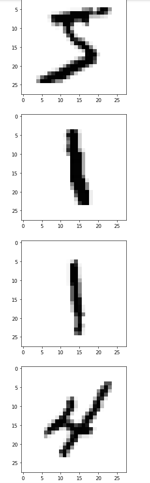
1.5 图像数据示例
运行程序:
# 示例
for i in range(10):
    img = train_imgs[i].reshape((28,28))
    plt.imshow(img, cmap="Greys")
    plt.show()
运行结果:
1.6 pickle包保存python对象
因为csv文件读取到内存比较慢,我们用pickle这个包来保存python对象(这里面python对象指的是numpy array格式的train_imgs, test_imgs, train_labels, test_labels)
运行程序:
import pickle

with open("D:\\pickled_mnist.pkl", "bw") as fh:
    data = (train_imgs,
            test_imgs,
            train_labels,
            test_labels)
    pickle.dump(data, fh)
2 构建神经网络并训练
2.1 读取pickle文件
运行程序:
import pickle

with open("D:\\19实验\\实验课大作业\\pickled_mnist.pkl", "br") as fh:
    data = pickle.load(fh)

train_imgs = data[0]
test_imgs = data[1]
train_labels = data[2]
test_labels = data[3]

train_labels_one_hot = (lable_range==train_labels).astype(float)
test_labels_one_hot = (label_range==test_labels).astype(float)


image_size = 28 # width and length
num_of_different_labels = 10 #  i.e. 0, 1, 2, 3, ..., 9
image_pixels = image_size * image_size
2.2 神经网络核心关键函数定义
运行程序:
import numpy as np

def sigmoid(x):
    return 1 / (1 + np.e ** -x)
##激活函数
activation_function = sigmoid

from scipy.stats import truncnorm
##数据标准化
def truncated_normal(mean=0, sd=1, low=0, upp=10):
    return truncnorm((low - mean) / sd,
                     (upp - mean) / sd,
                     loc=mean,
                     scale=sd)
##构建神经网络模型
class NeuralNetwork:

    def __init__(self,
                 num_of_in_nodes, #输入节点数
                 num_of_out_nodes, #输出节点数
                 num_of_hidden_nodes,#隐藏节点数
                 learning_rate):#学习率
        self.num_of_in_nodes = num_of_in_nodes
        self.num_of_out_nodes = num_of_out_nodes
        self.num_of_hidden_nodes = num_of_hidden_nodes
        self.learning_rate = learning_rate
        self.create_weight_matrices()
    #初始为一个隐藏节点
    def create_weight_matrices(self):#创建权重矩阵

       # A method to initialize the weight
        #matrices of the neural network#一种初始化神经网络权重矩阵的方法

        rad = 1 / np.sqrt(self.num_of_in_nodes)
        X = truncated_normal(mean=0, sd=1, low=-rad, upp=rad)  #形成指定分布
        self.weight_1 = X.rvs((self.num_of_hidden_nodes, self.num_of_in_nodes)) #rvs:产生服从指定分布的随机数

        rad = 1 / np.sqrt(self.num_of_hidden_nodes)
        X = truncated_normal(mean=0, sd=1, low=-rad, upp=rad)
        self.weight_2 = X.rvs((self.num_of_out_nodes, self.num_of_hidden_nodes)) #rvs: 产生服从指定分布的随机数


    def train(self, input_vector, target_vector):
      #
       # input_vector and target_vector can
        #be tuple, list or ndarray
        #

        input_vector = np.array(input_vector, ndmin=2).T#输入
        target_vector = np.array(target_vector, ndmin=2).T#输出

        output_vector1 = np.dot(self.weight_1, input_vector) #隐藏层值
        output_hidden = activation_function(output_vector1)#删除不激活

        output_vector2 = np.dot(self.weight_2, output_hidden)#输出
        output_network = activation_function(output_vector2)##删除不激活

        # calculate output errors:计算输出误差
        output_errors = target_vector - output_network

        # update the weights:更新权重
        tmp = output_errors * output_network * (1.0 - output_network)
        self.weight_2 += self.learning_rate  * np.dot(tmp, output_hidden.T)


        # calculate hidden errors:计算隐藏层误差
        hidden_errors = np.dot(self.weight_2.T, output_errors)

        # update the weights:
        tmp = hidden_errors * output_hidden * (1.0 - output_hidden)
        self.weight_1 += self.learning_rate * np.dot(tmp, input_vector.T)

    #测试集
    def run(self, input_vector):
        # input_vector can be tuple, list or ndarray
        input_vector = np.array(input_vector, ndmin=2).T


        output_vector = np.dot(self.weight_1, input_vector)
        output_vector = activation_function(output_vector)

        output_vector = np.dot(self.weight_2, output_vector)
        output_vector = activation_function(output_vector)

        return output_vector
    #判别矩阵
    def confusion_matrix(self, data_array, labels):
        cm = np.zeros((10, 10), int)
        for i in range(len(data_array)):
            res = self.run(data_array[i])
            res_max = res.argmax()
            target = labels[i][0]
            cm[res_max, int(target)] += 1
        return cm
     #精确度
    def precision(self, label, confusion_matrix):
        col = confusion_matrix[:, label]
        return confusion_matrix[label, label] / col.sum()
    #评估
    def evaluate(self, data, labels):
        corrects, wrongs = 0, 0
        for i in range(len(data)):
            res = self.run(data[i])
            res_max = res.argmax()
            if res_max == labels[i]:
                corrects += 1
            else:
                wrongs += 1
        return corrects, wrongs
2.3 神经网络模型定义
运行程序:
ANN = NeuralNetwork(num_of_in_nodes = image_pixels, #输入
                    num_of_out_nodes = 10, #输出节点数
                    num_of_hidden_nodes = 100,#隐藏节点
                    learning_rate = 0.1)#学习率
2.4 模型训练
2.4.1 预测概率
运行程序:
for i in range(len(train_imgs)):
    ANN.train(train_imgs[i], train_labels_one_hot[i])


for i in range(20):
    res = ANN.run(test_imgs[i])
    print(test_labels[i], np.argmax(res), np.max(res))
运行结果:
[7.] 7 0.9992648448921
[2.] 2 0.9040034245332168
[1.] 1 0.9992201001324703
[0.] 0 0.9923701545281887
[4.] 4 0.989297708155559
[1.] 1 0.9984582148795715
[4.] 4 0.9957673752296046
[9.] 9 0.9889417895800644
[5.] 6 0.5009071817613537
[9.] 9 0.9879513019542627
[0.] 0 0.9932950902790246
[6.] 6 0.9387061553685657
[9.] 9 0.9962530965286298
[0.] 0 0.9974524110371016
[1.] 1 0.9991354417269441
[5.] 5 0.7607733657668813
[9.] 9 0.9968080255475414
[7.] 7 0.9967748204232602
[3.] 3 0.8820920415159276
[4.] 4 0.9978584850755227
2.4.2 训练集正确率
运行程序:
corrects, wrongs = ANN.evaluate(train_imgs, train_labels)#训练集判别正确和错误数量
print("accuracy train: ", corrects / ( corrects + wrongs))##正确率
运行结果:
accuracy train: 0.9425333333333333
2.4.3 测试集正确率
运行程序:
corrects, wrongs = ANN.evaluate(test_imgs, test_labels)
print("accuracy: test", corrects / ( corrects + wrongs))#测试集正确率
运行结果:
accuracy: test 0.9412
2.4.4 训练集判别矩阵
运行程序:
cm = ANN.confusion_matrix(train_imgs, train_labels)
print(cm)   #训练集判别矩阵
运行结果:
[[5822    1   54   35   15   41   47   12   31   31]
 [   2 6638   62   31   17   24   21   64  163   14]
 [   6   19 5487   57   16    9    2   45   16    4]
 [   7   27   87 5773    3  130    3   16  148   67]
 [  11   11   68    8 5332   34   12   48   28   44]
 [  10    4    6   69    0 4952   34    5   32    5]
 [  31    5   53   19   49   96 5782    5   37    2]
 [   1    9   45   35    6    6    0 5812    5   28]
 [  20    9   70   32    9   37   15   11 5209    9]
 [  13   19   26   72  395   92    2  247  182 5745]]
2.4.5 不同数字预测精确率
运行程序:
for i in range(10):
    print("digit: ", i, "precision: ", ANN.precision(i, cm))
运行结果:
digit:  0 precision:  0.9829478304913051
digit:  1 precision:  0.9845743102936814
digit:  2 precision:  0.9209466263846928
digit:  3 precision:  0.9416082205186755
digit:  4 precision:  0.9127011297500855
digit:  5 precision:  0.9134845969378343
digit:  6 precision:  0.9770192632646164
digit:  7 precision:  0.9276935355147645
digit:  8 precision:  0.8902751666381815
digit:  9 precision:  0.9657085224407463
2.5 结果可视化
2.5.1 每次epoch训练预测情况
运行程序:
epochs = 30
train_acc=[]
test_acc=[]
NN = NeuralNetwork(num_of_in_nodes = image_pixels,
                   num_of_out_nodes = 10,
                   num_of_hidden_nodes = 100,
                   learning_rate = 0.1)

for epoch in range(epochs):
    print("epoch: ", epoch)
    for i in range(len(train_imgs)):
        NN.train(train_imgs[i],
                 train_labels_one_hot[i])

    corrects, wrongs = NN.evaluate(train_imgs, train_labels)
    print("accuracy train: ", corrects / ( corrects + wrongs))
    train_acc.append(corrects / ( corrects + wrongs))
    corrects, wrongs = NN.evaluate(test_imgs, test_labels)
    print("accuracy: test", corrects / ( corrects + wrongs))
    test_acc.append(corrects / ( corrects + wrongs))
运行结果:
epoch:  0
accuracy train:  0.94455
accuracy: test 0.9422
epoch:  1
accuracy train:  0.9628
accuracy: test 0.9579
epoch:  2
accuracy train:  0.9699
accuracy: test 0.9637
epoch:  3
accuracy train:  0.9761166666666666
accuracy: test 0.9649
epoch:  4
accuracy train:  0.979
accuracy: test 0.9662
epoch:  5
accuracy train:  0.9820833333333333
accuracy: test 0.9679
epoch:  6
accuracy train:  0.9838166666666667
accuracy: test 0.9697
epoch:  7
accuracy train:  0.9845666666666667
accuracy: test 0.97
epoch:  8
accuracy train:  0.9855333333333334
accuracy: test 0.9703
epoch:  9
accuracy train:  0.9868166666666667
accuracy: test 0.97
epoch:  10
accuracy train:  0.9878166666666667
accuracy: test 0.9714
epoch:  11
accuracy train:  0.98845
accuracy: test 0.9716
epoch:  12
accuracy train:  0.98905
accuracy: test 0.9721
epoch:  13
accuracy train:  0.9898166666666667
accuracy: test 0.9723
epoch:  14
accuracy train:  0.9903
accuracy: test 0.9722
epoch:  15
accuracy train:  0.9907666666666667
accuracy: test 0.9719
epoch:  16
accuracy train:  0.9910833333333333
accuracy: test 0.9715
epoch:  17
accuracy train:  0.9918
accuracy: test 0.9714
epoch:  18
accuracy train:  0.9924166666666666
accuracy: test 0.971
epoch:  19
accuracy train:  0.99265
accuracy: test 0.9712
epoch:  20
accuracy train:  0.9932833333333333
accuracy: test 0.972
epoch:  21
accuracy train:  0.9939333333333333
accuracy: test 0.9716
epoch:  22
accuracy train:  0.9944333333333333
accuracy: test 0.972
epoch:  23
accuracy train:  0.9948
accuracy: test 0.9719
epoch:  24
accuracy train:  0.9950833333333333
accuracy: test 0.9718
epoch:  25
accuracy train:  0.9950833333333333
accuracy: test 0.9722
epoch:  26
accuracy train:  0.99525
accuracy: test 0.9725
epoch:  27
accuracy train:  0.9955833333333334
accuracy: test 0.972
epoch:  28
accuracy train:  0.9958166666666667
accuracy: test 0.9717
epoch:  29
accuracy train:  0.9962666666666666
accuracy: test 0.9717
2.5.2 迭代30次正确率绘图
运行程序:
#正确率绘图
# matplotlib其实是不支持显示中文的 显示中文需要一行代码设置字体
import numpy as np
import matplotlib as mpl
import matplotlib.pyplot as plt
mpl.rcParams['font.family'] = 'SimHei'
plt.rcParams['axes.unicode_minus'] = False
import matplotlib.pyplot as plt
x=np.arange(1,31,1)
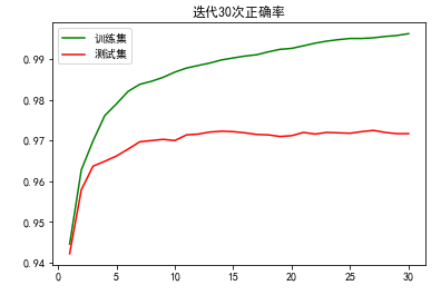
plt.title('迭代30次正确率')
plt.plot(x, train_acc, color='green', label='训练集')
plt.plot(x, test_acc, color='red', label='测试集')
plt.legend() # 显示图例
plt.show()
运行结果:
3 模型优化
3.1 调整神经元数量
3.1.1 每次epoch训练预测情况
运行程序:
##更换隐藏神经元数量为50
epochs = 50
train_acc=[]
test_acc=[]
NN = NeuralNetwork(num_of_in_nodes = image_pixels,
                   num_of_out_nodes = 10,
                   num_of_hidden_nodes = 50,
                   learning_rate = 0.1)

for epoch in range(epochs):
    print("epoch: ", epoch)
    for i in range(len(train_imgs)):
        NN.train(train_imgs[i],
                 train_labels_one_hot[i])

    corrects, wrongs = NN.evaluate(train_imgs, train_labels)
    print("accuracy train: ", corrects / ( corrects + wrongs))
    train_acc.append(corrects / ( corrects + wrongs))
    corrects, wrongs = NN.evaluate(test_imgs, test_labels)
    print("accuracy: test", corrects / ( corrects + wrongs))
    test_acc.append(corrects / ( corrects + wrongs))
运行结果:
epoch:  0
accuracy train:  0.93605
accuracy: test 0.935
epoch:  1
accuracy train:  0.95185
accuracy: test 0.9501
epoch:  2
accuracy train:  0.9570333333333333
accuracy: test 0.9526
epoch:  3
accuracy train:  0.9630833333333333
accuracy: test 0.9556
epoch:  4
accuracy train:  0.9640166666666666
accuracy: test 0.9556
epoch:  5
accuracy train:  0.9668333333333333
accuracy: test 0.957
epoch:  6
accuracy train:  0.96765
accuracy: test 0.957
epoch:  7
accuracy train:  0.9673166666666667
accuracy: test 0.9566
epoch:  8
accuracy train:  0.96875
accuracy: test 0.9559
epoch:  9
accuracy train:  0.97145
accuracy: test 0.957
epoch:  10
accuracy train:  0.974
accuracy: test 0.9579
epoch:  11
accuracy train:  0.9730666666666666
accuracy: test 0.9569
epoch:  12
accuracy train:  0.9730166666666666
accuracy: test 0.9581
epoch:  13
accuracy train:  0.9747666666666667
accuracy: test 0.959
epoch:  14
accuracy train:  0.9742166666666666
accuracy: test 0.9581
epoch:  15
accuracy train:  0.97615
accuracy: test 0.9596
epoch:  16
accuracy train:  0.9759
accuracy: test 0.9586
epoch:  17
accuracy train:  0.9773166666666666
accuracy: test 0.9596
epoch:  18
accuracy train:  0.9778833333333333
accuracy: test 0.9606
epoch:  19
accuracy train:  0.9789166666666667
accuracy: test 0.9589
epoch:  20
accuracy train:  0.9777333333333333
accuracy: test 0.9582
epoch:  21
accuracy train:  0.9774
accuracy: test 0.9573
epoch:  22
accuracy train:  0.9796166666666667
accuracy: test 0.9595
epoch:  23
accuracy train:  0.9792666666666666
accuracy: test 0.959
epoch:  24
accuracy train:  0.9804333333333334
accuracy: test 0.9591
epoch:  25
accuracy train:  0.9806
accuracy: test 0.9589
epoch:  26
accuracy train:  0.98105
accuracy: test 0.9596
epoch:  27
accuracy train:  0.9806833333333334
accuracy: test 0.9587
epoch:  28
accuracy train:  0.9809833333333333
accuracy: test 0.9595
epoch:  29
accuracy train:  0.9813333333333333
accuracy: test 0.9595
3.1.2 正确率绘图
运行程序:
#正确率绘图
# matplotlib其实是不支持显示中文的 显示中文需要一行代码设置字体
import numpy as np
import matplotlib as mpl
import matplotlib.pyplot as plt
mpl.rcParams['font.family'] = 'SimHei'
plt.rcParams['axes.unicode_minus'] = False   # 步骤二(解决坐标轴负数的负号显示问题)

import matplotlib.pyplot as plt

x=np.arange(1,31,1)

plt.title('神经元数量为50时正确率')
plt.plot(x, train_acc, color='green', label='训练集')
plt.plot(x, test_acc, color='red', label='测试集')

plt.legend() # 显示图例
plt.show()
运行结果:

3.2 更换隐藏层层数
3.2.1 每次epoch训练预测情况
运行程序:
#隐藏层层数为2
class NeuralNetwork:

    def __init__(self,
                 num_of_in_nodes, #输入节点数
                 num_of_out_nodes, #输出节点数
                 num_of_hidden_nodes1,#隐藏第一层节点数
                 num_of_hidden_nodes2,#隐藏第二层节点数
                 learning_rate):#学习率
        self.num_of_in_nodes = num_of_in_nodes
        self.num_of_out_nodes = num_of_out_nodes
        self.num_of_hidden_nodes1 = num_of_hidden_nodes1
        self.num_of_hidden_nodes2 = num_of_hidden_nodes2
        self.learning_rate = learning_rate
        self.create_weight_matrices()
    #初始为一个隐藏节点
    def create_weight_matrices(self):#创建权重矩阵

        #A method to initialize the weight
        #matrices of the neural network#一种初始化神经网络权重矩阵的方法

        rad = 1 / np.sqrt(self.num_of_in_nodes)
        X = truncated_normal(mean=0, sd=1, low=-rad, upp=rad)  #形成指定分布
        self.weight_1 = X.rvs((self.num_of_hidden_nodes1, self.num_of_in_nodes)) #rvs:产生服从指定分布的随机数

        rad = 1 / np.sqrt(self.num_of_hidden_nodes1)
        X = truncated_normal(mean=0, sd=1, low=-rad, upp=rad)
        self.weight_2 = X.rvs((self.num_of_hidden_nodes2, self.num_of_hidden_nodes1)) #rvs: 产生服从指定分布的随机数

        rad = 1 / np.sqrt(self.num_of_hidden_nodes2)
        X = truncated_normal(mean=0, sd=1, low=-rad, upp=rad)
        self.weight_3 = X.rvs((self.num_of_out_nodes, self.num_of_hidden_nodes2)) #rvs: 产生服从指定分布的随机数
    def train(self, input_vector, target_vector):

        #input_vector and target_vector can
        #be tuple, list or ndarray


        input_vector = np.array(input_vector, ndmin=2).T#输入
        target_vector = np.array(target_vector, ndmin=2).T#输出

        output_vector1 = np.dot(self.weight_1, input_vector) #隐藏层值
        output_hidden1 = activation_function(output_vector1)#删除不激活

        output_vector2 = np.dot(self.weight_2, output_hidden1)#输出
        output_hidden2 = activation_function(output_vector2)#删除不激活

        output_vector3 = np.dot(self.weight_3, output_hidden2)#输出
        output_network = activation_function(output_vector3)##删除不激活


        # calculate output errors:计算输出误差
        output_errors = target_vector - output_network

        # update the weights:更新权重
        tmp = output_errors * output_network * (1.0 - output_network)
        self.weight_3 += self.learning_rate  * np.dot(tmp, output_hidden2.T)

        hidden1_errors = np.dot(self.weight_3.T, output_errors)

        tmp = hidden1_errors * output_hidden2 * (1.0 - output_hidden2)
        self.weight_2 += self.learning_rate  * np.dot(tmp, output_hidden1.T)


        # calculate hidden errors:计算隐藏层误差
        hidden_errors = np.dot(self.weight_2.T, hidden1_errors)

        # update the weights:
        tmp = hidden_errors * output_hidden1 * (1.0 - output_hidden1)
        self.weight_1 += self.learning_rate * np.dot(tmp, input_vector.T)

    #测试集
    def run(self, input_vector):
        # input_vector can be tuple, list or ndarray
        input_vector = np.array(input_vector, ndmin=2).T


        output_vector = np.dot(self.weight_1, input_vector)
        output_vector = activation_function(output_vector)

        output_vector = np.dot(self.weight_2, output_vector)
        output_vector = activation_function(output_vector)

        output_vector = np.dot(self.weight_3, output_vector)
        output_vector = activation_function(output_vector)
        return output_vector
    #判别矩阵
    def confusion_matrix(self, data_array, labels):
        cm = np.zeros((10, 10), int)
        for i in range(len(data_array)):
            res = self.run(data_array[i])
            res_max = res.argmax()
            target = labels[i][0]
            cm[res_max, int(target)] += 1
        return cm
     #精确度
    def precision(self, label, confusion_matrix):
        col = confusion_matrix[:, label]
        return confusion_matrix[label, label] / col.sum()
    #评估
    def evaluate(self, data, labels):
        corrects, wrongs = 0, 0
        for i in range(len(data)):
            res = self.run(data[i])
            res_max = res.argmax()
            if res_max == labels[i]:
                corrects += 1
            else:
                wrongs += 1
        return corrects, wrongs

##迭代30次
epochs = 30
train_acc=[]
test_acc=[]
NN = NeuralNetwork(num_of_in_nodes = image_pixels,
                   num_of_out_nodes = 10,
                   num_of_hidden_nodes1 = 100,
                   num_of_hidden_nodes2 = 100,
                   learning_rate = 0.1)

for epoch in range(epochs):
    print("epoch: ", epoch)
    for i in range(len(train_imgs)):
        NN.train(train_imgs[i],
                 train_labels_one_hot[i])

    corrects, wrongs = NN.evaluate(train_imgs, train_labels)
    print("accuracy train: ", corrects / ( corrects + wrongs))
    train_acc.append(corrects / ( corrects + wrongs))
    corrects, wrongs = NN.evaluate(test_imgs, test_labels)
    print("accuracy: test", corrects / ( corrects + wrongs))
    test_acc.append(corrects / ( corrects + wrongs))
运行结果:
epoch:  0
accuracy train:  0.8972333333333333
accuracy: test 0.9005
epoch:  1
accuracy train:  0.8891833333333333
accuracy: test 0.8936
epoch:  2
accuracy train:  0.9146833333333333
accuracy: test 0.9182
epoch:  3
D:\ananconda\lib\site-packages\ipykernel_launcher.py:5: RuntimeWarning: overflow encountered in power
  """
accuracy train:  0.8974833333333333
accuracy: test 0.894
epoch:  4
accuracy train:  0.8924166666666666
accuracy: test 0.8974
epoch:  5
accuracy train:  0.91295
accuracy: test 0.914
epoch:  6
accuracy train:  0.9191166666666667
accuracy: test 0.9205
epoch:  7
accuracy train:  0.9117666666666666
accuracy: test 0.9162
epoch:  8
accuracy train:  0.9220333333333334
accuracy: test 0.9222
epoch:  9
accuracy train:  0.9113833333333333
accuracy: test 0.9112
epoch:  10
accuracy train:  0.9134333333333333
accuracy: test 0.911
epoch:  11
accuracy train:  0.9112166666666667
accuracy: test 0.9103
epoch:  12
accuracy train:  0.914
accuracy: test 0.9126
epoch:  13
accuracy train:  0.9206833333333333
accuracy: test 0.9214
epoch:  14
accuracy train:  0.90945
accuracy: test 0.9073
epoch:  15
accuracy train:  0.9225166666666667
accuracy: test 0.9287
epoch:  16
accuracy train:  0.9226
accuracy: test 0.9205
epoch:  17
accuracy train:  0.9239833333333334
accuracy: test 0.9202
epoch:  18
accuracy train:  0.91925
accuracy: test 0.9191
epoch:  19
accuracy train:  0.9223166666666667
accuracy: test 0.92
epoch:  20
accuracy train:  0.9113
accuracy: test 0.9084
epoch:  21
accuracy train:  0.9241666666666667
accuracy: test 0.925
epoch:  22
accuracy train:  0.9236333333333333
accuracy: test 0.9239
epoch:  23
accuracy train:  0.9301166666666667
accuracy: test 0.9259
epoch:  24
accuracy train:  0.9195166666666666
accuracy: test 0.9186
epoch:  25
accuracy train:  0.9200833333333334
accuracy: test 0.9144
epoch:  26
accuracy train:  0.9204833333333333
accuracy: test 0.9186
epoch:  27
accuracy train:  0.9288666666666666
accuracy: test 0.9259
epoch:  28
accuracy train:  0.9293
accuracy: test 0.9282
epoch:  29
accuracy train:  0.9254666666666667
accuracy: test 0.9242
3.2.2 正确率绘图
运行程序:
#正确率绘图
# matplotlib其实是不支持显示中文的 显示中文需要一行代码设置字体
import numpy as np
import matplotlib as mpl
import matplotlib.pyplot as plt
mpl.rcParams['font.family'] = 'SimHei'
plt.rcParams['axes.unicode_minus'] = False # 步骤二(解决坐标轴负数的负号显示问题)
import matplotlib.pyplot as plt
x=np.arange(1,31,1)
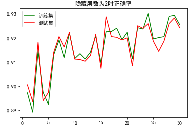
plt.title('隐藏层数为2时正确率')
plt.plot(x, train_acc, color='green', label='训练集')
plt.plot(x, test_acc, color='red', label='测试集')
plt.legend() # 显示图例
plt.show()
运行结果: