GCN-LSTM 可以学习参考 英文内容部分源自youtube的教学视频 自己跟着英文敲的
给定一辆出租车行驶时在某个时间段的速度,下一个时刻速度会是多少?这是一个时间序列回归预测问题。获得了若干时间点的速度,目标是预测出租车速度序列中的下一个具体数值,但是,如果模型没有获取速度序列的上下文,这个预测是不可能的。例如,表1的出租车运行速度中,40km/h后面是三个不同的速度值。但随着输入序列的不断增加,下一个时刻的速度变得越来越容易预测。
长期短期记忆网络(LSTM)是为输入数据是有序时间序列的现实场景应用设计的。其中,来自序列中待预测值前若干个时刻的信息可能对训练效果来说不可或缺。 LSTM 是一种循环神经网络(RNN),它是每次训练都把上一步的输出作为下一步的输入的网络。LSTM神经网络就像其他种类的神经网络一样,它的节点使用若干数据进行输入,网络内部执行若干个周期的计算,更新并返回输出值。
LSTM 中的节点使用内部状态作为数据记忆存储单元,可以在多个时间步长上存储和获取信息。输入值、先前输出和内部状态都用于节点计算。计算结果不仅用于提供输出值,还用于更新状态。
LSTM 节点像普通的BP神经网络节点一样,具有确定在计算中使用输入数据的权重的参数,但 LSTM 还具有称为门的参数,它控制了节点内的信息流。这些门的参数包括训练产生的权重和偏差,这意味着LSTM的行为取决于输入。例如,如果LSTM需要预测上一时刻是0km/h的下一时刻信息,那么,除非出租车是启动的状态,否则大概率下一时刻速度仍然是0km/h。但是,如果给 LSTM输入上一个时刻的车速为40km/h,神经网络就可能需要输入更多的数据才能预测下一个时刻的状态。
LSTM 神经网络包含3种门控单元,分别为输入门、和输出门和遗忘门。其中,遗忘门的作用是操控网络下一次更新状态时需要丢弃的信息数量。遗忘门的状态更新公式为:
输入门的作用是控制和选择神经网络本次输入的数据保留在单元状态中的部分。输入门的状态更新公式为:
输出门的作用是控制和选择神经网络当前单元状态的数据中要输出的部分。输出门的状态更新公式为:
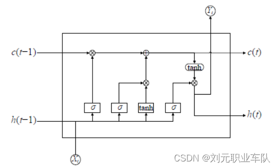
公式中,……
LSTM 的节点相比于一般的RNN节点更复杂,因为门也可以选择有多少当前信息应该被记忆并保存,以及有多少输出取决于当前计算与保存的信息。所以, LSTM 克服了学习时间序列数据中复杂的相互依赖关系的难题。
Given the speed of a taxi in a certain period of time, what will the speed be at the next moment? This is a time series regression forecasting problem. The speed at several points in time is obtained, and the goal is to predict the next specific value in the taxi speed sequence, but this prediction is not possible if the model does not have access to the context of the speed sequence. For example, in the taxi running speed in Table 1, 40km/h is followed by three different speed values. But as the input sequence continues to grow, the velocity of the next moment becomes more and more predictable.
Long Short Term Memory (LSTM) networks are designed for real-world applications where the input data is an ordered time series. Among them, information from several moments before the value to be predicted in the sequence may be indispensable for the training effect. LSTM is a kind of recurrent neural network (RNN), which is a network that uses the output of the previous step as the input of the next step for each training. The LSTM neural network is like other kinds of neural networks, its nodes use some data for input, and the network performs several cycles of calculations, updates and returns the output value.
Nodes in LSTMs use internal states as data memory storage units and can store and retrieve information over multiple time steps. Input values, previous outputs, and internal states are all used for node computation. Calculation results are used not only to provide output values, but also to update state.
LSTM nodes, like normal BP neural network nodes, have parameters that determine the weights of the input data used in the computation, but LSTMs also have parameters called gates, which control the flow of information within the node. The parameters of these gates include weights and biases resulting from training, which means that the behavior of the LSTM depends on the input. For example, if LSTM needs to predict the information of the next moment when the last moment is 0km/h, then unless the taxi is in the state of starting, there is a high probability that the speed at the next moment will still be 0km/h. However, if the speed of the vehicle at the previous moment is 40km/h as input to the LSTM, the neural network may need to input more data to predict the state of the next moment.
The LSTM neural network contains three kinds of gating units, namely the input gate, the output gate and the forgetting gate. Among them, the function of the forget gate is to control the amount of information that needs to be discarded when the network updates the state next time. The state update formula of the forget gate is: The function of the input gate is to control and select the part of the input data of the neural network that remains in the unit state. The state update formula of the input gate is: The function of the output gate is to control and select the part of the data to be output from the current unit state of the neural network. The state update formula of the output gate is:
LSTM nodes are more complex than general RNN nodes, because the gate can also choose how much current information should be memorized and saved, and how much output depends on the current computed and saved information. So, LSTM overcomes the difficulty of learning complex interdependencies in time series data.
original
If we’re looking at a sequence of letters, what’s likely to come next? This is a prediction problem. We’re given a letter, the goal is to predict the next letter in the sequence, but this prediction is impossible without the context of the sequence of letters. For example, here …. Is followed by three different letters. But in context, the next letter becomes easier and easier to predict as a sequence progresses. Long short term memory networks, or LSTM networks, are designed for applications where the input is an ordered sequence where information from earlier in the sequence may be important. LSTM is a type of recurrent network which are networks that reuse the output from a previous step as an input for the next step. Like all neural networks, the node performs a calculation using the inputs and returns an output value. In a recurrent network, this output is then used along with the next element as the inputs for the next step, and so on. In an LSTM, the nodes are recurrent, but they also have an internal state. The node uses an internal state as a working memory space, which means information can be stored and retrieved over many time steps. The input value, previous output and the internal state are all use in the nodes calculations. The results of the calculations are used not only to provide an output value but also to update the state. Like any neural network, LSTM nodes have parameters that determine how the inputs are used in the calculations, but LSTMs also have parameters known as gates that control the flow of information within the node. In particular, how much the safe state information is used as an input to the calculations? These gate parameters are weights and biases which means the behavior depends on the inputs. So for example, when LSTM receives an input of .. , it might need some more passed information. Similarly, there are gates to control how much of the current information is saved to the state and how much the output is determined by the current calculation versus the saved information. So LSTM nodes are certainly more complicated than regular recurrent nodes. They makes LSTM better at learning the complex interdependencies in sequences of data. Ultimately, they’re still just a node with a bunch of parameters, and these parameters are learned during training just like with any other neural networks.
如果获取了某城市区域每条公路某时间段的人流量、车流量和车辆速度等信息,希望训练一个模型,输入其他信息以预测车辆速度,数据分析师们可以简单地选定特征值和目标值,建立支持向量机(SVM)、随机森林或BP神经网络模型进行回归预测。但是,这些算法没有考虑到现实场景中城市道路与道路之间的连接关系。
在图数据结构中传递消息的算法是一种有创新价值的思想。图中的节点有自己的邻接节点,节点可以沿着互相的连接来传递数据。这可以被认为是分两个步骤发生的。首先,节点将向其邻接节点发送自己储存的权重信息,其他节点收集他们收到的数据,并使用它们来更新自己的权重,理解它周围的环境。
图神经网络(GCN) 可以理解为一种迭代式传播消息的算法。 首先,选择图中的一个节点,获取这个节点和它的邻接节点的权重属性。然后,设置一个聚合函数,如平均值或最大值,记录在这个节点中。接下来,将这个新的值输入一个神经网络的全连接层,进行特征提取,并对它应用一个激活函数(如ReLU)。这个全连接层的输出是该节点更新后的权重。该节点新的权重不仅是其邻接节点的平均值,而是通过了指定非线性函数的平均值。GCN会遍历整张图,对图中的每个节点都进行这个操作。每个节点都通过边获取它的邻接节点的权重,进行聚合函数计算,将计算结果向量通过神经网络传递输出,计算获取更新后的这一节点的新向量。如果GCN拥有多层,在总的结构上,这与普通的全连接BP神经网络相似。算法所做的只是重复相同的过程,对上一层输出的更新权重的较小的图再次更新权重,输出新的图。 但是,与全连接神经网络不同的是,在GCN的每一层的开始都有一个预处理步骤,让节点收集其所有邻接节点的值,并聚合它们。
GCN的输出与大多数神经网络原理类似。如果想使用关于城市公路的信息预测车辆的平均速度,我们可以将GCN输出维度设置为 1,并设置回归计算常用的损失函数(如MSE),训练数据集。训练完成后,给定新的特征信息,即可输出预测值。
If information such as pedestrian volume, traffic volume and average vehicle speed for a period of time of each highway in a certain urban area is obtained, and it is wished to train a model, input other information to predict vehicle speed, data analysts can simply select feature values and target values, and build support vector machine (SVM), random forest or BP neural network model for regression prediction. However, these algorithms do not take into account the connections between roads and roads in real-world scenarios.
Algorithms for passing messages in graph data structures are an innovative idea. Nodes in the graph have their own neighbors, and nodes can pass data along the connections to each other. This can be thought of as happening in two steps. First, a node will send its own stored weight information to its neighbors, and other nodes collect the data they receive and use them to update their own weights and understand the environment around it.
Graph Neural Network (GCN) can be understood as an algorithm that iteratively propagates messages. First, select a node in the graph and get the weight attribute of this node and its adjacent nodes. Then, set an aggregate function, such as mean or max, to be recorded in this node. Next, feed this new value into a fully connected layer of a neural network, perform feature extraction, and apply an activation function (such as ReLU) to it. The output of this fully connected layer is the updated weight of the node. The new weight of this node is not only the average of its neighbors, but the average of the specified nonlinear function. GCN traverses the entire graph, doing this for every node in the graph. Each node obtains the weight of its adjacent nodes through the edge, performs aggregation function calculation, transmits the calculation result vector through the neural network, and calculates and obtains the updated new vector of this node. If the GCN has multiple layers, in the overall structure, it is similar to the ordinary fully connected BP neural network. All the algorithm does is repeat the same process, update the weights again for the smaller graph with the updated weights output by the previous layer, and output a new graph. However, unlike a fully-connected neural network, there is a preprocessing step at the beginning of each layer of GCNs that lets a node collect the values of all its neighbors and aggregate them.
The output of GCN is similar in principle to most neural networks. If we want to predict the average speed of vehicles using information about urban roads, we can set the GCN output dimension to 1, select a common loss function (like MSE) on GCN regression model on the training dataset. After the training is completed, given new feature information, the predicted value can be output.
original
The idea of passing message in a graph data structure is a really powerful concept because a lot of the graph algorithms can be understood from that perspective. In a nutshell, the idea is that a node in a graph can send and receive message along its connections with its neighbors. This can be thought of as happening in two steps. First, nodes will send out message about itself to its neighbors and next nodes collect the neighbor messages they receive and use them in some way to update itself and understand its environment. In a fraud use case, you can see how fraud labels can propagate through the graph by continually passing and collecting messages. This is the essence of label propagation algorithms. Here’s a little schematic showing how this works conceptually in a graph that connects accounts with their shared attributes like IP address and credit card numbers. In label propagation, each node in the graph starts with an initial state and that state is updated by receiving messages from the other nodes that it’s connected to. This repeats in the next iteration except each node now starts with its updated state which takes its neighbors into consideration. Think of this as smoothing the label information across a neighborhood. GCNs can be understood as a simple message passing algorithm, but whereas label propagation just passes messages about the label value. GCNs do this for an entire vector of input data. So, an account doesn’t just tell us neighbors it’s fraud or not, but its credit card is from the US and my IP address is from Vietnam and my billing address is in Ireland, and whatever else you know about the account. If flayed propagation is label smoothing in a neighborhood, think GCN as feature smoothing. Let’s make this concrete by talking through a simple calculation and a GCN layer. For any node in the graph, first get all of the attribute vectors of tis connected nodes, and apply some aggregation functions like an average. Next, pass this average vector through a dense neural network layer, which is a fancy way of saying multiply it by some matrix and apply an activation function. The output of this dense layer is the new vector representation of the node. So, now the node isn’t just an average of its neighbors but the average of its neighbors passed through some nonlinear function. This process must be done for every node in the graph. Each node collects messages from its neighbors aggregates those messages and passes the resulting vector through a standard neural network to get a new vector that represents the node. The node is then represents by this new vector. For the second layer, all you do is repeat the same process except the input od the input is the updates vectors from the first layer. This is similar in concept to a traditional fully connected neural network, the raw input goes into the first layer, and the output of the first layer is the input layer of the second layer, and so on. The same is true with GCNs except there’s a pre-processing step at the beginning of each layer where a node has to first get the values of all its neighbors and aggregate them. If want to classify each node like fraud or not fraud, we can set this output dimensionality to 1 and use a typical binary cross-entropy loss function with back propagation to train all of out parameters.






![P1308 [NOIP2011 普及组] 统计单词数————C++](https://img-blog.csdnimg.cn/5232a83cf1ff4062af86acb710379379.png)

