线性回归案例

一、初始化方法

1.对数据进行预处理模块，调用prepare_for_training方法，得到返回值data_processed, features_mean, features_deviation
2.得到所有的特征个数，即data的特征维数的列(行shape[0]，列shape[1])
3.初始化参数矩阵

 # data:数据 labels:有监督的标签 polynomial_degree、sinusoid_degree、normalize_data: 三个都是预训练需要用到的参数
    def __init__(self, data , labels,polynomial_degree = 0,sinusoid_degree =0,normalize_data=True):
        # data_processed, features_mean, features_deviation 是 prepare_for_training() 方法的三个返回值
        (data_processed,
         features_mean,
         features_deviation) = prepare_for_training(data,polynomial_degree=0,sinusoid_degree=0,normalize_data=True)
        self.data = data_processed
        self.labels = labels
        self.features_mean = features_mean
        self.features_deviation = features_deviation
        self.polynomial_degree = polynomial_degree
        self.sinusoid_degree = sinusoid_degree
        self.normalize_data = normalize_data

        num_features = self.data.shape[1] # 获得数据的特征数目 即data的特征维数的列(行shape[0]，列shape[1])
        self.theta = np.zeros((num_features,1)) # 参数θ 个数等于num_features  (num_features,1)转换成矩阵形式

预训练模块

"""Prepares the dataset for training"""
import numpy as np
from .normalize import normalize
from .generate_sinusoids import generate_sinusoids
from .generate_polynomials import generate_polynomials

def prepare_for_training(data, polynomial_degree=0, sinusoid_degree=0, normalize_data=True):
    # 计算样本总数
    num_examples = data.shape[0]
    data_processed = np.copy(data)

    # 预处理
    features_mean = 0
    features_deviation = 0
    data_normalized = data_processed
    if normalize_data:
        (
            data_normalized,
            features_mean,
            features_deviation
        ) = normalize(data_processed)

        data_processed = data_normalized

    # 特征变换sinusoidal
    if sinusoid_degree > 0:
        sinusoids = generate_sinusoids(data_normalized, sinusoid_degree)
        data_processed = np.concatenate((data_processed, sinusoids), axis=1)

    # 特征变换polynomial
    if polynomial_degree > 0:
        polynomials = generate_polynomials(data_normalized, polynomial_degree, normalize_data)
        data_processed = np.concatenate((data_processed, polynomials), axis=1)

    # 加一列1
    data_processed = np.hstack((np.ones((num_examples, 1)), data_processed))

    return data_processed, features_mean, features_deviation

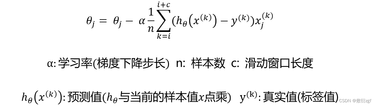
二、定义计算梯度的方法

按照小批量梯度下降法计算：

# 定义每一步梯度下降的计算过程
    def gradient_step(self,alpha): # alpha 
    	'''
        梯度下降参数更新计算方法
        :param alpha: 学习率
        :return: 
   	 	'''
        # 样本个数 即data的特征维数的行shape[0]
        num_examples = self.data.shape[0]
        # 预测值
        prediction = LinearRegression.hypothesis(self.data,self.theta)
        delta = prediction - self.labels # 预测值 - 真实值
        # 初始化theta
        theta = self.theta
        # 更新theta 参照上述公式 delta.T 按照转置进行矩阵运算
        theta = theta - alpha * ( 1 / num_examples ) * (np.dot(delta.T , self.data)).T
        self.theta = theta
    # 定义静态方法hypothesis 计算预测值
    @staticmethod
    def hypothesis(data, theta):
        predictions = np.dot(data, theta) # 预测值为data 与 theta 做点乘运算
        return predictions

三、定义损失计算方法

损失函数采用均方误差

    def cost_function(self,data,labels):
        '''
        损失计算方法
        :param data: 样本数据
        :param labels: 真实值
        :return:cost[0][0] 损失值
        '''
        num_examples = data.shape[0] # 样本数目
        delta = LinearRegression.hypothesis(self.data,self.theta) - labels
        # 损失函数计算采用均方误差
        cost = (1/2) * np.dot(delta.T , delta) / num_examples
        return cost[0][0] # 损失值位于二维数组[0][0],只需要返回损失值

四、定义训练函数

# 定义训练方法 alpha:学习率(步长) num_iterations:迭代次数
    def train(self,alpha,num_iterations = 500):
        '''
        训练模块，执行梯度下降
        :param alpha:
        :param num_iterations:
        :return:
        '''
        cost_history = self.gradient_descent(alpha,num_iterations) # 调用该方法不仅可以得到每一步的损失值，而且对参数theta进行了更新
        return self.theta ,cost_history

# 定义梯度下降计算方法
    def gradient_descent(self,alpha,num_iterations):
        '''
        实际迭代模块，迭代num_iterations次
        :param alpha:
        :param num_iterations:
        :return:cost_history
        '''
        cost_history = [] # 列表存放损失
        for _ in range(num_iterations) :
            self.gradient_step(alpha) # 调用每一步具体的计算梯度方法
            cost_history.append(self.cost_function(self.data,self.labels))
        return cost_history # 返回每一步的损失值列表

五、定义获得损失值的方法

不仅仅是训练数据需要计算损失值，之后再进行预测时也需要计算损失值，传入得参数不一样，因此需要重新写一个获得损失值得方法，同时也方便后续进行可视化等操作。

    def get_cost(self,data,labels):
        data_processed = prepare_for_training(data,
                                              self.polynomial_degree,
                                              self.sinusoid_degree,
                                              self.normalize_data
                                              )[0]
        return self.cost_function(data_processed ,labels)

六、定义预测函数

用训练的参数模型，预测得到回归结果

    def predict(self,data):
        '''
        用训练的参数模型，预测得到回归结果
        :param data
        '''
        data_processed = prepare_for_training(data,
                                              self.polynomial_degree,
                                              self.sinusoid_degree,
                                              self.normalize_data
                                              )[0]
        predictions = LinearRegression.hypothesis(data_processed, self.theta)
        return predictions

那么以上线性回归模型的整体框架就已经搭建完成啦！
接下来利用实际数据进行模型验证

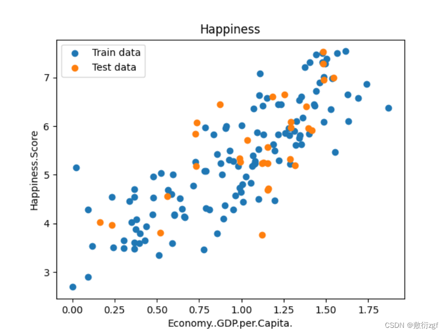
七、数据与标签定义

首先通过read_csv方法加载数据，接着通过matplotlib相关绘图方法绘制图像

import numpy as np
import pandas as pd
import matplotlib.pyplot as plt
from linear_regression import LinearRegression

data = pd.read_csv('./data/world-happiness-report-2017.csv')
# 将数据划分成训练集和测试集
train_data = data.sample(frac= 0.8) # 80% 作为训练集
test_data = data.drop(train_data.index) # 将训练集索引对应的数据删除，剩下的即为测试集 也就是数据的20%
# 定义标签
input_param_name= 'Economy..GDP.per.Capita.'
output_param_name= 'Happiness.Score'

x_train = train_data[[input_param_name]].values # 将数据转换成numpy的ndarray格式(多维数组)
y_train = train_data[[output_param_name]].values

x_test = test_data[[input_param_name]].values
y_test = test_data[[output_param_name]].values

plt.scatter(x_train,y_train,label = 'Train data')
plt.scatter(x_test,y_test,label = 'Test data')
plt.xlabel(input_param_name)
plt.ylabel(output_param_name)
plt.title('Happiness')
plt.legend()
plt.show()

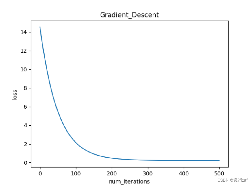
八、训练线性回归模型

# 模型迭代次数
num_iterations = 500
# 学习率
learning_rate = 0.01
linear_regression = LinearRegression(x_train, y_train)
(theta,cost_history) = linear_regression.train(learning_rate,num_iterations)
print('开始时的损失:',cost_history[0])
print('训练后的损失:',cost_history[-1])
plt.plot(range(num_iterations),cost_history)
plt.xlabel('num_iterations')
plt.ylabel('loss')
plt.title('Gradient_Descent')
plt.show()

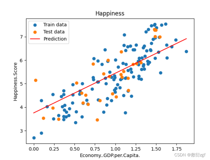
九、得到线性回归方程

predicitions_num = 100
# linspace在指定的大间隔内(x_train.min(),x_train.max())，返回固定间隔的数据。返回predicitions_num个等间距的样本
x_predictions = np.linspace(x_train.min(),x_train.max(),predicitions_num).reshape(predicitions_num,1)
y_predictions = linear_regression.predict(x_predictions) # 调用预测函数

plt.scatter(x_train,y_train,label = 'Train data')
plt.scatter(x_test,y_test,label = 'Test data')
plt.plot(x_predictions,y_predictions,'r',label = 'Prediction')
plt.xlabel(input_param_name)
plt.ylabel(output_param_name)
plt.title('Happiness')
plt.legend()
plt.show()

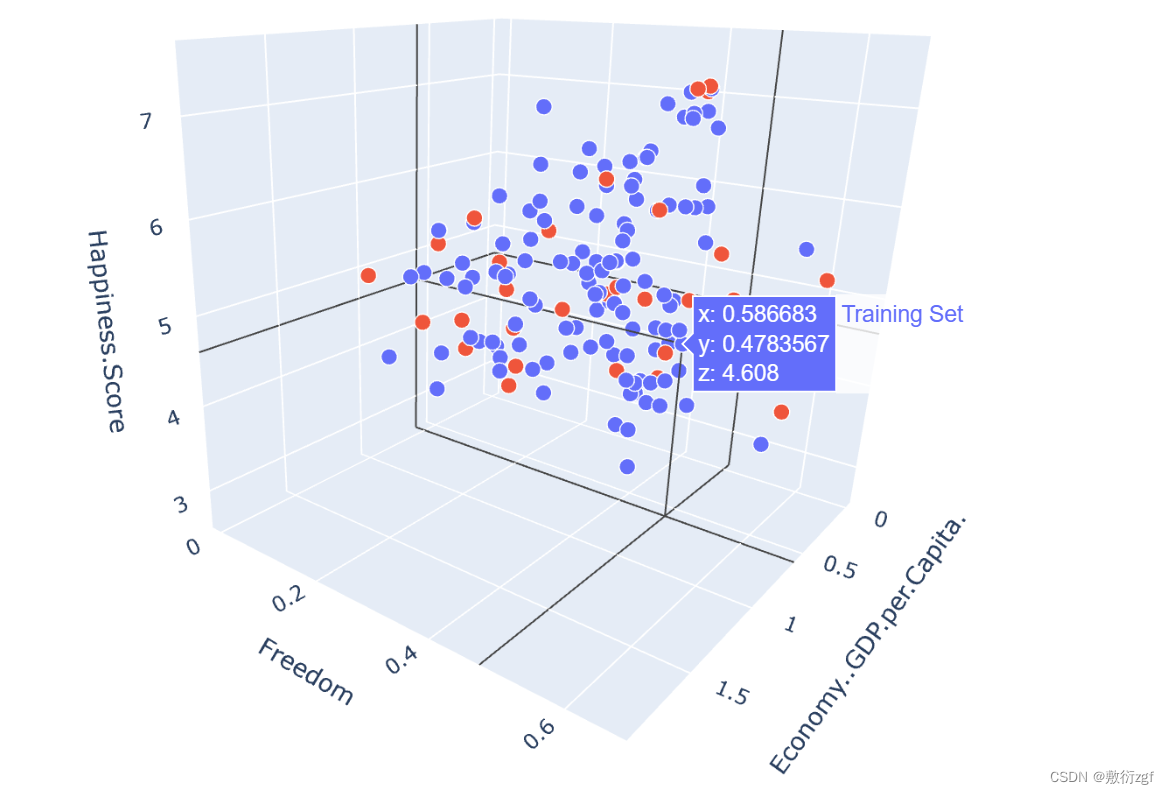
十、多特征线性回归模型

导包 & 读入数据

# 导入第三方库
import numpy as np
import pandas as pd
import matplotlib.pyplot as plt
import plotly # 用于机器学习、数据挖掘等领域的数据可视化包
import plotly.graph_objs as go

plotly.offline.init_notebook_mode()
from linear_regression import LinearRegression

# 加载数据
data = pd.read_csv('./data/world-happiness-report-2017.csv')

划分数据集

# 划分数据集
train_data = data.sample(frac=0.8)
test_data = data.drop(train_data.index)

# 定义标签
input_param_name_1 = 'Economy..GDP.per.Capita.'
input_param_name_2 = 'Freedom'
output_param_name = 'Happiness.Score'

# 得到训练集数据
x_train = train_data[[input_param_name_1 , input_param_name_2]].values
y_train = train_data[[output_param_name]].values

# 得到测试集数据
x_test = test_data[[input_param_name_1 , input_param_name_2]].values
y_test = test_data[[output_param_name]].values

配置绘图

# Configure the plot with training dataset 配置训练集数据进行绘图
plot_training_trace = go.Scatter3d(
    x = x_train[:,0].flatten(), # 第一维特征
    y = x_train[:,1].flatten(), # 第二维特征
    z = y_train.flatten(), # 真实值
    name = 'Training Set',
    mode= 'markers',
    marker = {
        'size' : 10 ,
        'opacity' : 1 ,
        'line' : {
            'color' : 'rgb(255,255,255)',
            'width' : 1
        }
    },
)
# Configure the plot with test dataset 配置测试集数据进行绘图
plot_test_trace = go.Scatter3d(
    x = x_test[:,0].flatten(), # 第一维特征
    y = x_test[:,1].flatten(), # 第二维特征
    z = y_test.flatten(), # 真实值
    name = 'Test Set',
    mode= 'markers',
    marker = {
        'size' : 10 ,
        'opacity' : 1 ,
        'line' : {
            'color' : 'rgb(255,255,255)',
            'width' : 1
        }
    },
)
plot_layout = go.Layout(
    title = 'Date Sets',
    scene = {
        'xaxis' : {'title' : input_param_name_1},
        'yaxis' : {'title' : input_param_name_2},
        'zaxis' : {'title' : output_param_name}
    },
    margin={'l':0,'r':0,'b':0,'t':0}
)
plot_data = [plot_training_trace , plot_test_trace]
plot_figure = go.Figure(data = plot_data, layout = plot_layout)
plotly.offline.plot(plot_figure)

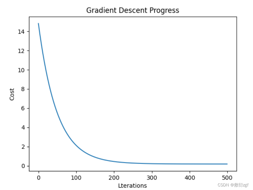
训练多维特征线性回归模型

num_iterations = 500
learning_rate = 0.01
polynomial_degree = 0
sinusoid_degree = 0
linear_regression = LinearRegression(x_train,y_train,polynomial_degree,sinusoid_degree)
# 调用训练模型方法
(theta , cost_history) = linear_regression.train(
    learning_rate ,
    num_iterations
)
print('开始损失',cost_history[0])
print('结束损失',cost_history[-1])

plt.plot(range(num_iterations) , cost_history)
plt.xlabel('Lterations')
plt.ylabel('Cost')
plt.title('Gradient Descent Progress')
plt.show()

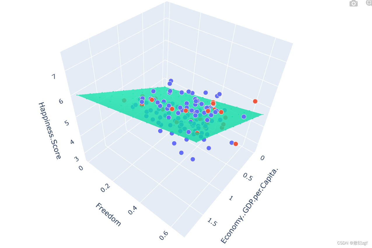
绘制回归面图

predictions_num  = 10
x_min = x_train[:,0].min()
x_max = x_train[:,0].max()

y_min = x_train[:,1].min()
y_max = x_train[:,1].max()

x_axis = np.linspace(x_min , x_max , predictions_num)
y_axis = np.linspace(y_min , y_max , predictions_num)

x_predictions = np.zeros((predictions_num * predictions_num, 1))
y_predictions = np.zeros((predictions_num * predictions_num, 1))

x_y_index = 0
for x_index , x_value in enumerate(x_axis):
    for y_index , y_value in enumerate(y_axis):
        x_predictions[x_y_index] = x_value
        y_predictions[x_y_index] = y_value
        x_y_index += 1

z_predictions = linear_regression.predict(np.hstack((x_predictions , y_predictions)))
plot_predictions_trace = go.Scatter3d(
    x = x_predictions.flatten(),
    y = y_predictions.flatten(),
    z = z_predictions.flatten(),
    name = 'Prediction Plane',
    mode = 'markers',
    marker={
        'size':1,
    },
    opacity = 0.8,
    surfaceaxis = 2 ,
)
plot_data = [plot_training_trace , plot_test_trace , plot_predictions_trace]
plot_figure = go.Figure(data = plot_data , layout= plot_layout)
plotly.offline.plot(plot_figure)