ggplot基本作图
1 条形图
library(ggplot2)
ggplot(biopics) +
  geom_histogram(aes(x = year_release),binwidth=1,fill="gray")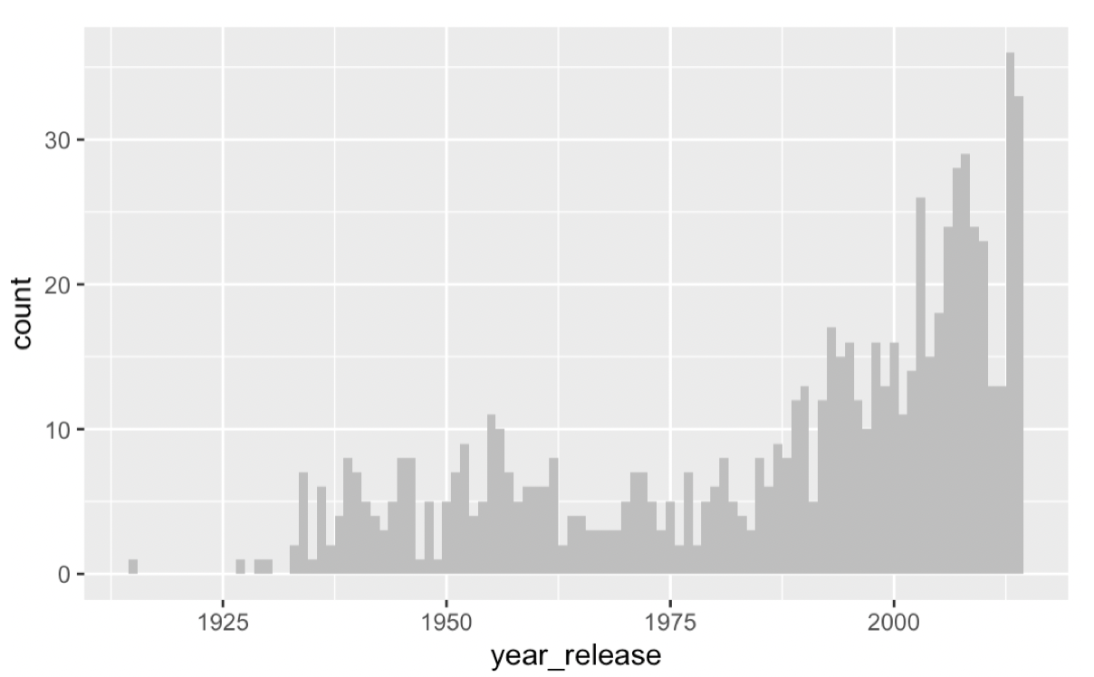
2 堆砌柱状图
ggplot(biopics, aes(x=year_release)) +
  geom_bar(aes(fill=subject_sex))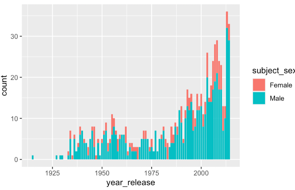
3 堆砌比例柱状图
ggplot(biopics, aes(x=year_release)) +
  geom_bar(aes(fill=subject_sex),position = 'fill')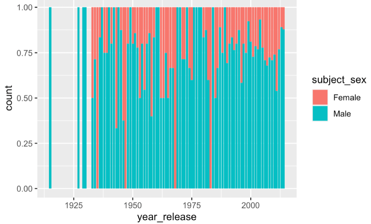
4 马赛克图
library(vcd)
bio_ques_d <- biopics[,c(11,13)]
bio_ques_d$subject_race <- ifelse(is.na(bio_ques_d$subject_race ), "missing",
                                 ifelse(bio_ques_d$subject_race == "White","White", "nonwhite"))
biq_ques_d_table <- table(bio_ques_d$subject_race,bio_ques_d$subject_sex)
mosaicplot(biq_ques_d_table)
5 双散点图
process_var <- c('v32', 'v33', 'v34', 'v35', 'v36', 'v37')
for (i in c(1:6)){
  var_clean <- paste(process_var[i],'clean',sep = '_')
  data[,var_clean] <- ifelse(data[,process_var[i]] == 'trust completely',1,
                             ifelse(data[,process_var[i]] == 'trust somewhat',2,
                                    ifelse(data[,process_var[i]] == 'do not trust very much',3,
                                           ifelse(data[,process_var[i]] == 'do not trust at all',4,NA))))
}
data$intp.trust <- rowSums(data[,c(438:443)],na.rm = TRUE)
data$intp.trust <- data$intp.trust/6
ggplot(data[data$country == 'Iceland',], aes(x=confidence, y=intp.trust, colour=v225)) + geom_point()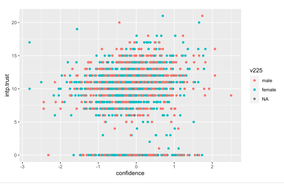
6 双密度图
ggplot(data=start_s_country_data) +
  geom_density(aes(x=residual,color=as.factor(v225),))

## 自定义图例的情况
ggplot(data=data) +
  geom_density(aes(x=LW, color = "LW")) +
  geom_density(aes(x=LP, color = "LP")) +
  labs(title="") +
  xlab("Value") +
  theme(legend.title=element_blank(),
        legend.position = c(0.9, 0.9))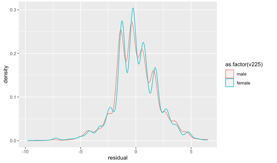
ggplot(data ) +
  geom_point(aes(x = No.education, y=Median.year.of.schooling)) +
  geom_smooth(aes(x = No.education, y=Median.year.of.schooling), method = 'lm') +
  theme_classic()
7 双折线图与多图展示
library(dplyr)
library(devtools)
library(cowplot)

plot_grid(plot1,plot3,plot5,plot2,plot4,plot6,ncol=3,nrow=2)
bio_ques_f <- biopics[,c(4,11,13)]
bio_ques_f$subject_race <- ifelse(is.na(bio_ques_f$subject_race ), "missing",
                                 ifelse(bio_ques_f$subject_race == "White","White", "nonwhite"))

planes <- group_by(bio_ques_f, year_release, subject_race, subject_sex)
bio_ques_f_summary <- summarise(planes, count = n())
planes <- group_by(bio_ques_f,year_release)
bio_ques_f_year<- summarise(planes,count_year = n())

bio_ques_f_summary <- left_join(bio_ques_f_summary,bio_ques_f_year,c("year_release" = "year_release"))
bio_ques_f_summary$prop <- bio_ques_f_summary$count / bio_ques_f_summary$count_year

data_missing_female <- subset(bio_ques_f_summary,with(bio_ques_f_summary,(subject_race == 'missing') & (subject_sex == 'Female')))
data_missing_male <- subset(bio_ques_f_summary,with(bio_ques_f_summary,(subject_race == 'missing') & (subject_sex == 'Male')))
data_nonwhite_female <- subset(bio_ques_f_summary,with(bio_ques_f_summary,(subject_race == 'nonwhite') & (subject_sex == 'Female')))
data_nonwhite_male <- subset(bio_ques_f_summary,with(bio_ques_f_summary,(subject_race == 'nonwhite') & (subject_sex == 'Male')))
data_white_female <- subset(bio_ques_f_summary,with(bio_ques_f_summary,(subject_race == 'White') & (subject_sex == 'Female')))
data_white_male <- subset(bio_ques_f_summary,with(bio_ques_f_summary,(subject_race == 'White') & (subject_sex == 'Male')))


plot1 <- ggplot(data_missing_female)+
           geom_line(aes(x=year_release,y=count),color="red") +
           geom_line(aes(x=year_release,y=prop),color="blue") +
           labs(title="missing and female")
plot2 <- ggplot(data_missing_male)+
           geom_line(aes(x=year_release,y=count),color="red") +
           geom_line(aes(x=year_release,y=prop),color="blue") +
           labs(title="missing and male")
plot3 <- ggplot(data_nonwhite_female)+
           geom_line(aes(x=year_release,y=count),color="red") +
           geom_line(aes(x=year_release,y=prop),color="blue") +
           labs(title="nonwhite and female")
plot4 <- ggplot(data_nonwhite_male)+
           geom_line(aes(x=year_release,y=count),color="red") +
           geom_line(aes(x=year_release,y=prop),color="blue") +
           labs(title="nonwhite and male")
plot5 <- ggplot(data_white_female)+
           geom_line(aes(x=year_release,y=count),color="red") +
           geom_line(aes(x=year_release,y=prop),color="blue") +
           labs(title="white and female")
plot6 <- ggplot(data_white_male)+
           geom_line(aes(x=year_release,y=count),color="red") +
           geom_line(aes(x=year_release,y=prop),color="blue") +
           labs(title="white and male")

plot_grid(plot1,plot3,plot5,plot2,plot4,plot6,ncol=3,nrow=2)
ggplot作图美化
1 标题居中
ggplot(data_selected, aes(x=AREA.NAME)) +
  geom_bar(aes(fill=year)) +
  labs(title = 'The bar plot of AREA.NAME') +
  theme_classic() +
  theme(plot.title = element_text(hjust = 0.5))
2 X轴标签旋转
ggplot(data_selected, aes(x=AREA.NAME)) +
  geom_bar(aes(fill=year)) +
  labs(title = 'The bar plot of AREA.NAME') +
  theme_classic() +
  theme(plot.title = element_text(hjust = 0.5)) +
  theme(axis.text.x=element_text(face="bold",size=8,angle=270,color="black"))
3 变更label名
ggplot(data=data) +
  geom_line(aes(x=index,y=data,group=line,color=result)) +
  theme_classic() +
  scale_colour_manual(values=c("red", "blue"), labels=c("lose", "win"))
ggforce
ggforce能对绘制的图增加聚类图层,包括圆形、椭圆形、方形能多种。
North_latitude <- c(47.5, 52.3, 54.8, 48.4, 54.2,
                    54.8, 54.4, 48.8, 50.5, 52.7,
                    46.5, 46.9, 45.1, 45.9, 50.7,
                    48.5, 48.3, 48.1, 48.8, 49.4)
Elevation <- c(2, 1, 1, 2, 1,
               1, 1, 2, 2, 1,
               2, 2, 2, 2, 1,
               2, 2, 1, 1, 1)
Temperature <- c(39.27, 39.00, 38.35, 37.58, 39.38,
                 39.05, 39.65, 38.66, 37.97, 40.10,
                 37.05, 37.19, 36.92, 36.70, 38.01,
                 37.26, 36.97, 36.95, 37.68, 37.55)
data <- data.frame(North_latitude = North_latitude,
                   Elevation = Elevation,
                   Temperature = Temperature)
data$Elevation <- as.factor(data$Elevation)
dim(data)
library(ggplot2)
library(ggforce)
ggplot(data=data,aes(x=North_latitude,y=Temperature,color=Elevation))+
geom_point()+
geom_mark_circle(aes(fill=Elevation),alpha=0.4)+
theme_classic() +
labs(title = 'The relationship between latitude and temperature') +
theme(plot.title = element_text(hjust = 0.5))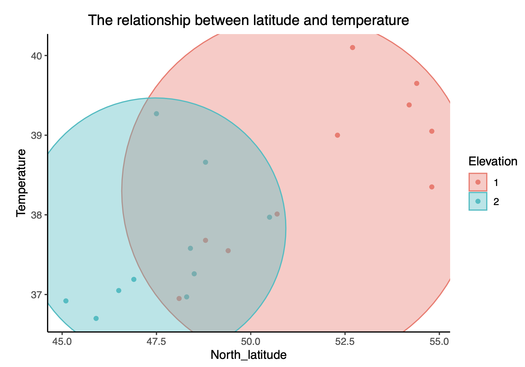
地理位置图
library(ggplot2)
library(viridis)
library(cvTools)
library(dplyr)

data <- read.csv("Reef_Check_with_cortad_variables_with_annual_rate_of_SST_change.csv")

world_map <- map_data("world")
ggplot() +
  geom_polygon(data =world_map, aes(x=long, y = lat, group = group), fill="grey", alpha=0.3) +
  geom_point(data =data, alpha = 0.2, aes(y=Latitude.Degrees, x= Longitude.Degrees , size=Average_bleaching, color=Average_bleaching))  + scale_colour_viridis() + theme_minimal()
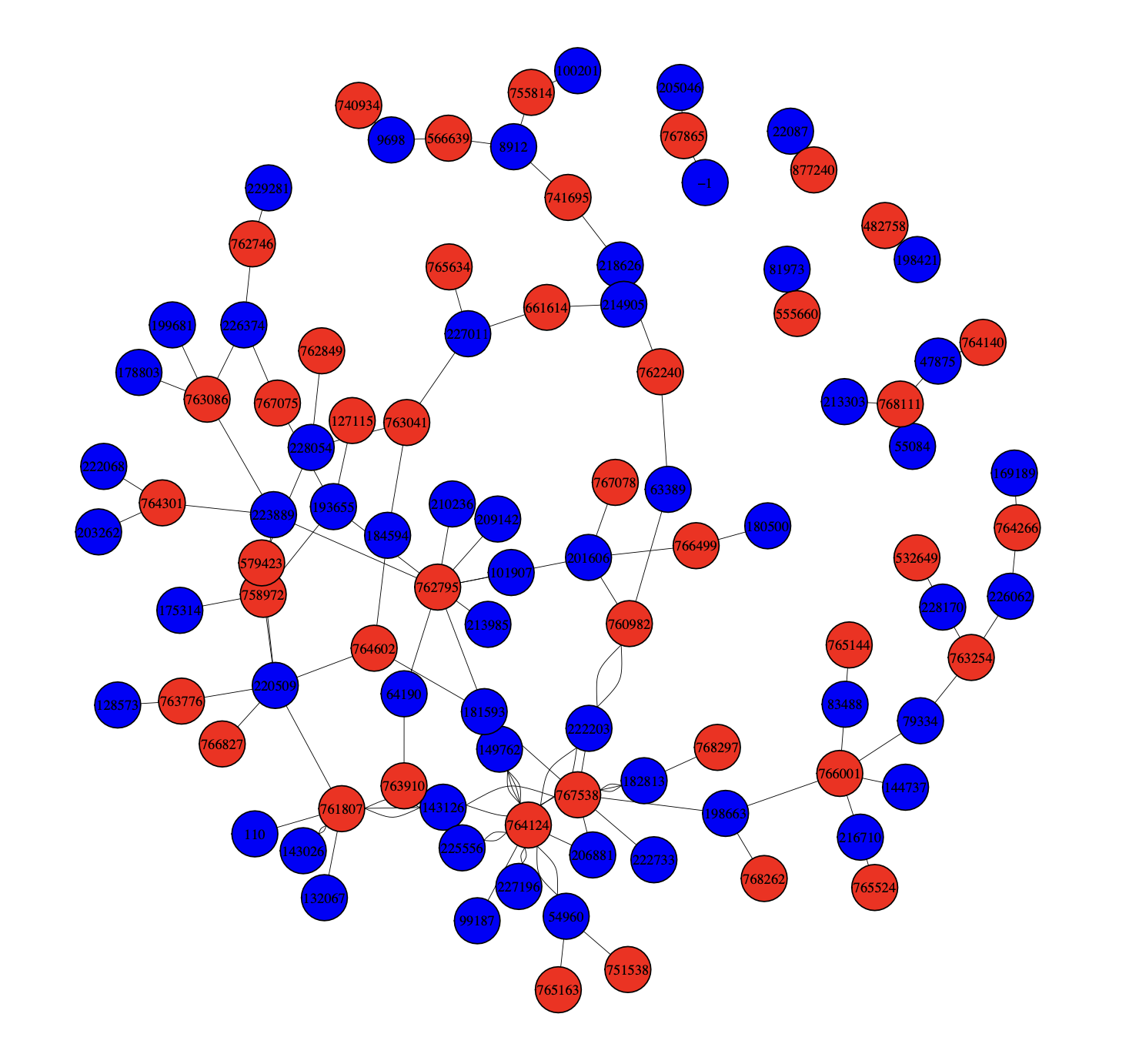
igraph网络图
library(igraph)

webforum_graph <- webforum[webforum$Date > as.Date("2010-12-01"), ]
webforum_graph <- webforum_graph[webforum_graph$Date < as.Date("2010-12-31"), ]

# generate node dataframe
AuthorID <- unique(as.numeric(webforum_graph$AuthorID))
ThreadID <- unique(as.numeric(webforum_graph$ThreadID))
name <- c(AuthorID, ThreadID)
type <- c(rep("Author", length(AuthorID)) , rep("Thread", length(ThreadID)))
webforum_node <- data.frame(name = name, type = type)

# generate edge dataframe
webforum_graph <- webforum_graph[,c("AuthorID", "ThreadID")]

# generate graph dataframe
graph <- graph_from_data_frame(webforum_graph, directed = FALSE, vertices=webforum_node)


set.seed(30208289)

plot(graph,
     layout= layout.fruchterman.reingold,
     vertex.size=10,
     vertex.shape="circle",
     vertex.color=ifelse(V(graph)$type == "Thread", "red", "blue"),
     vertex.label=NULL,
     vertex.label.cex=0.7,
     vertex.label.color='black',
     vertex.label.dist=0,
     edge.arrow.size=0.2,
     edge.width = 0.5,
     edge.label=V(graph)$year,
     edge.label.cex=0.5,
     edge.color="black")