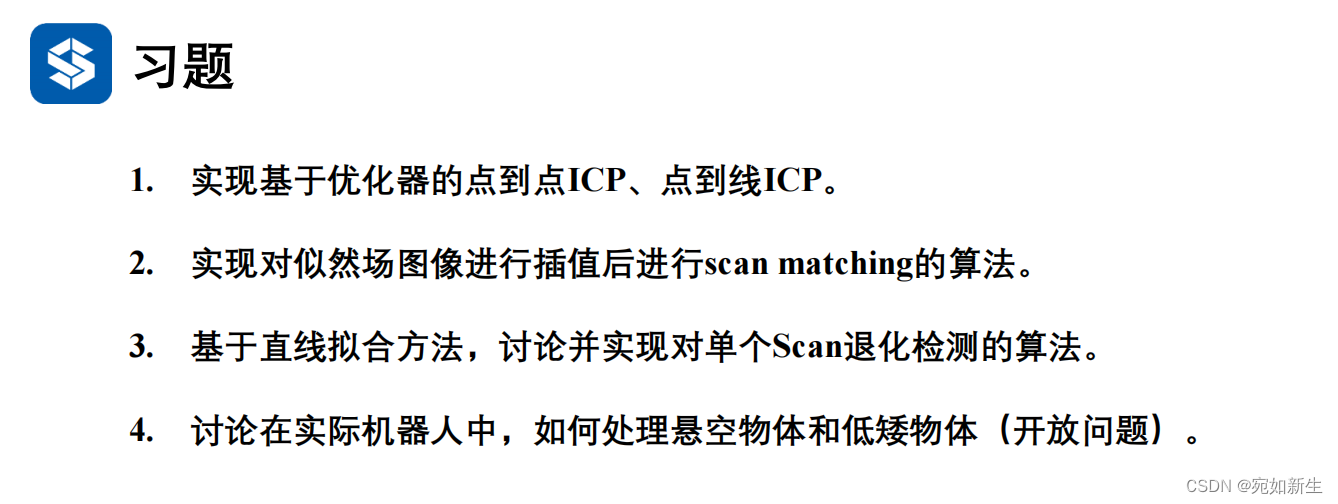
目录
- 1. 基于优化的点到点/线的配准
- 2. 对似然场图像进行插值,提高匹配精度
- 3. 对二维激光点云中会对SLAM功能产生退化场景的检测
- 4. 在诸如扫地机器人等这样基于2D激光雷达导航的机器人,如何处理悬空/低矮物体
- 5. 也欢迎大家来我的读书号--过千帆,学习交流。
1. 基于优化的点到点/线的配准
这里实现了基于g2o优化器的优化方法。
图优化中涉及两个概念-顶点和边。我们的优化变量认为是顶点,误差项就是边。我们通过g2o声明一个图模型,然后往图模型中添加顶点和与顶点相关联的边,再选定优化算法(比如LM)就可以进行优化了。想熟悉g2o的小伙伴们感兴趣的话,可以到这个链接看一下。
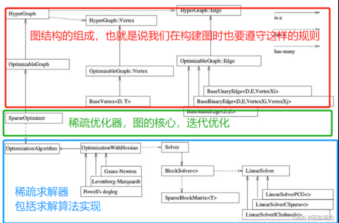
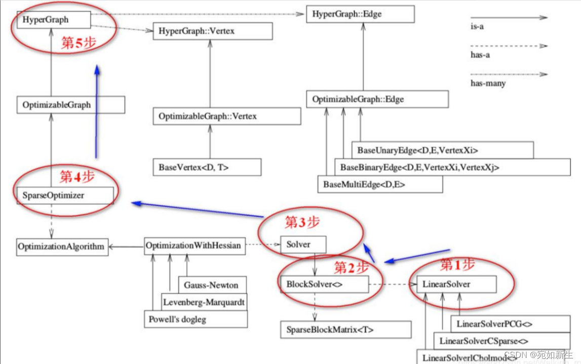
g2o的基本框架和编程套路如下图:
基于g2o的点对点的配准算法代码实现如下:
bool Icp2d::AlignWithG2oP2P(SE2& init_pose)
{
    double rk_delta = 0.8;    // 核函数阈值
    float max_dis2 = 0.01;    // 最近邻时的最远距离(平方)
    int min_effect_pts = 20;  // 最小有效点数

    // 构建图优化,先设定g2o
    typedef g2o::BlockSolver<g2o::BlockSolverTraits<3, 2>> BlockSolverType;  // 每个误差项优化变量维度为3, 误差值维度是2
    typedef g2o::LinearSolverDense<BlockSolverType::PoseMatrixType> LinearSolverType; // 线性求解器类型
    // 梯度下降方法,可以从GN, LM, DogLeg 中选
    auto solver = new g2o::OptimizationAlgorithmLevenberg(
            g2o::make_unique<BlockSolverType>(g2o::make_unique<LinearSolverType>()));

    g2o::SparseOptimizer optimizer;   // 图模型
    optimizer.setAlgorithm(solver);   // 设置求解器
    optimizer.setVerbose(false);       // 打开调试输出

    // 往图中添加顶点
    VertexSE2 *v = new VertexSE2(); // 新建SE2位姿顶点
    v->setId(0);                    // 设置顶点的id
    v->setEstimate(init_pose);      // 设置顶点的估计值为初始位姿
    optimizer.addVertex(v);         // 将顶点添加到优化器中

    // 往图中添加边
    int effective_num = 0;  // 有效点数
    // 遍历source
    for (size_t i = 0; i < source_scan_->ranges.size(); ++i)
    {
        float range = source_scan_->ranges[i];
        if (range < source_scan_->range_min || range > source_scan_->range_max)
        {
            continue;
        }

        float angle = source_scan_->angle_min + i * source_scan_->angle_increment;
        float theta = v->estimate().so2().log();
        Vec2d pw = v->estimate() * Vec2d(range * std::cos(angle), range * std::sin(angle));
        Point2d pt;
        pt.x = pw.x();
        pt.y = pw.y();

        // 最近邻
        std::vector<int> nn_idx;
        std::vector<float> dis;
        kdtree_.nearestKSearch(pt, 1, nn_idx, dis);

        if (nn_idx.size() > 0 && dis[0] < max_dis2)
        {
            effective_num++;
            Vec2d qw = Vec2d(target_cloud_->points[nn_idx[0]].x, target_cloud_->points[nn_idx[0]].y);   // 当前激光点在目标点云中的最近邻点坐标
            auto *edge = new EdgeIcpP2P(range, angle, theta);   // 构建约束边
            edge->setVertex(0, v);                   // 设置连接的顶点
            edge->setMeasurement(qw);                // 观测,即最近邻
            edge->setInformation(Mat2d::Identity()); // 观测为2维点坐标,因此信息矩阵需设为2x2单位矩阵
            auto rk = new g2o::RobustKernelHuber;    // Huber鲁棒核函数
            rk->setDelta(rk_delta);                  // 设置阈值
            edge->setRobustKernel(rk);               // 为边设置鲁棒核函数
            optimizer.addEdge(edge);                 // 将约束边添加到优化器中
        }
    }

    if (effective_num < min_effect_pts) {
        return false;
    }

    // 执行优化
    optimizer.initializeOptimization(); // 初始化优化器
    optimizer.optimize(10);             // 优化

    init_pose = v->estimate();

    LOG(INFO) << "g2o estimated pose: " << v->estimate().translation().transpose() << ", theta: " << v->estimate().so2().log();
    return true;
}
效果展示:

基于g2o的点对线的配准算法代码实现如下:
bool Icp2d::AlignWithG2oP2Plane(SE2& init_pose)
{
    double rk_delta = 0.8;    // 核函数阈值
    float max_dis2 = 0.01;    // 最近邻时的最远距离(平方)
    int min_effect_pts = 20;  // 最小有效点数

    // 构建图优化,先设定g2o
    typedef g2o::BlockSolver<g2o::BlockSolverTraits<3, 1>> BlockSolverType;  // 每个误差项优化变量维度为3, 误差值维度是1
    typedef g2o::LinearSolverDense<BlockSolverType::PoseMatrixType> LinearSolverType; // 线性求解器类型
    // 梯度下降方法,可以从GN, LM, DogLeg 中选
    auto solver = new g2o::OptimizationAlgorithmLevenberg(
            g2o::make_unique<BlockSolverType>(g2o::make_unique<LinearSolverType>()));

    g2o::SparseOptimizer optimizer;   // 图模型
    optimizer.setAlgorithm(solver);   // 设置求解器
    optimizer.setVerbose(true);       // 打开调试输出

    // 往图中添加顶点
    VertexSE2 *v = new VertexSE2(); // 新建SE2位姿顶点
    v->setId(0);                    // 设置顶点的id
    v->setEstimate(init_pose);      // 设置顶点的估计值为初始位姿
    optimizer.addVertex(v);         // 将顶点添加到优化器中

    // 往图中添加边
    int effective_num = 0;  // 有效点数
    // 遍历source
    for (size_t i = 0; i < source_scan_->ranges.size(); ++i)
    {
        float range = source_scan_->ranges[i];
        if (range < source_scan_->range_min || range > source_scan_->range_max)
        {
            continue;
        }

        float angle = source_scan_->angle_min + i * source_scan_->angle_increment;
        float theta = v->estimate().so2().log();
        Vec2d pw = v->estimate() * Vec2d(range * std::cos(angle), range * std::sin(angle));
        Point2d pt;
        pt.x = pw.x();
        pt.y = pw.y();

        // 查找5个最近邻
        std::vector<int> nn_idx;
        std::vector<float> dis;
        kdtree_.nearestKSearch(pt, 5, nn_idx, dis);

        std::vector<Vec2d> effective_pts;  // 有效点
        for (int j = 0; j < nn_idx.size(); ++j)
        {
            if (dis[j] < max_dis2)
            {
                effective_pts.emplace_back(
                    Vec2d(target_cloud_->points[nn_idx[j]].x, target_cloud_->points[nn_idx[j]].y));
            }
        }

        if (effective_pts.size() < 3)
        {
            continue;
        }

        // 拟合直线,组装J、H和误差
        Vec3d line_params;
        if (math::FitLine2D(effective_pts, line_params)) {
            effective_num++;
            auto *edge = new EdgeIcpP2Plane(range, angle, theta, line_params);   // 构建约束边
            edge->setVertex(0, v);                   // 设置连接的顶点
            edge->setInformation(Eigen::Matrix<double, 1, 1>::Identity()); // 误差为1维
            auto rk = new g2o::RobustKernelHuber;    // Huber鲁棒核函数
            rk->setDelta(rk_delta);                  // 设置阈值
            edge->setRobustKernel(rk);               // 为边设置鲁棒核函数
            optimizer.addEdge(edge);                 // 将约束边添加到优化器中
        }
    }

    if (effective_num < min_effect_pts)
    {
        return false;
    }

    // 执行优化
    optimizer.initializeOptimization(); // 初始化优化器
    optimizer.optimize(10);             // 优化10次

    init_pose = v->estimate();

    LOG(INFO) << "g2o estimated pose: " << v->estimate().translation().transpose() << ", theta: " << v->estimate().so2().log();
    return true;
}
其中,直线拟合的代码为: 其中,直线拟合的代码为: 其中,直线拟合的代码为:
template <typename S>
bool FitLine2D(const std::vector<Eigen::Matrix<S, 2, 1>>& data, Eigen::Matrix<S, 3, 1>& coeffs) {
    if (data.size() < 2) {
        return false;
    }

    Eigen::MatrixXd A(data.size(), 3);
    for (int i = 0; i < data.size(); ++i) {
        A.row(i).head<2>() = data[i].transpose();
        A.row(i)[2] = 1.0;
    }

    Eigen::JacobiSVD svd(A, Eigen::ComputeThinV);
    coeffs = svd.matrixV().col(2);
    return true;
}
效果展示:

2. 对似然场图像进行插值,提高匹配精度
高博书中分别实现了基于g2o和手写高斯牛顿两种方法,其中手写高斯牛顿法中没有使用插值,在g2o方法中用到了插值。这里直接将其挪用到手写高斯牛顿法中。所以这里不做赘述,只来介绍一下双线性插值的过程。
// bilinear interpolation
template <typename T>
inline float GetPixelValue(const cv::Mat& img, float x, float y) {
    // boundary check
    if (x < 0) x = 0;
    if (y < 0) y = 0;
    if (x >= img.cols) x = img.cols - 1;
    if (y >= img.rows) y = img.rows - 1;
    const T* data = &img.at<T>(floor(y), floor(x));
    float xx = x - floor(x);
    float yy = y - floor(y);
    return float((1 - xx) * (1 - yy) * data[0] + xx * (1 - yy) * data[1] + (1 - xx) * yy * data[img.step / sizeof(T)] +
                 xx * yy * data[img.step / sizeof(T) + 1]);
}
双线性插值的过程如图:
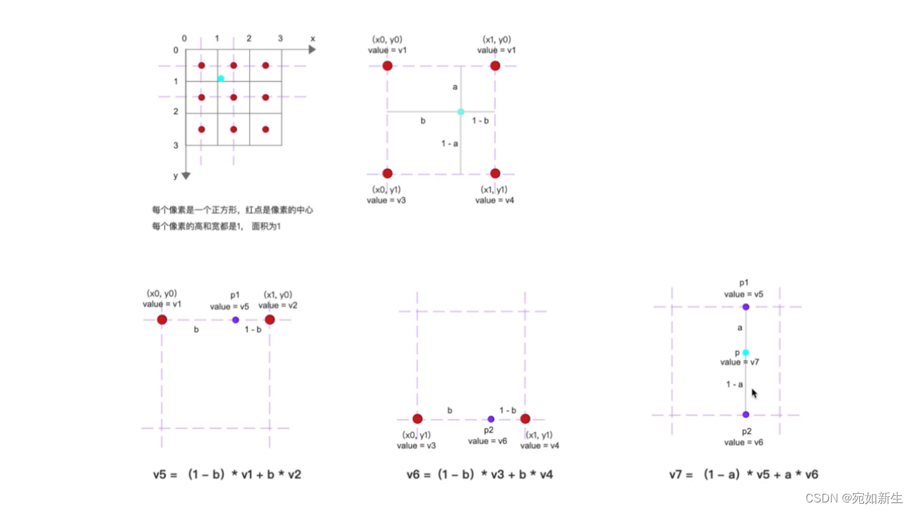
对应到程序中:
a = y y ; a=yy; a=yy;
b = x x ; b=xx; b=xx;
v 1 = d a t a [ 0 ] ; v1=data[0]; v1=data[0];
v 2 = d a t a [ 1 ] ; v2=data[1]; v2=data[1];
v 3 = d a t a [ i m g . s t e p / s i z e o f ( T ) ] ; v3=data[img.step / sizeof(T)]; v3=data[img.step/sizeof(T)];
v 4 = d a t a [ i m g . s t e p / s i z e o f ( T ) + 1 ] ; v4=data[img.step / sizeof(T) + 1]; v4=data[img.step/sizeof(T)+1];
===================================>可得:
v 7 = f l o a t ( ( 1 − x x ) ∗ ( 1 − y y ) ∗ d a t a [ 0 ] + x x ∗ ( 1 − y y ) ∗ d a t a [ 1 ] + ( 1 − x x ) ∗ y y ∗ d a t a [ i m g . s t e p / s i z e o f ( T ) ] + x x ∗ y y ∗ d a t a [ i m g . s t e p / s i z e o f ( T ) + 1 ] ) ; v7=float((1 - xx) * (1 - yy) * data[0] + xx * (1 - yy) * data[1] + (1 - xx) * yy * data[img.step / sizeof(T)] + xx * yy * data[img.step / sizeof(T) + 1]); v7=float((1−xx)∗(1−yy)∗data[0]+xx∗(1−yy)∗data[1]+(1−xx)∗yy∗data[img.step/sizeof(T)]+xx∗yy∗data[img.step/sizeof(T)+1]);
效果展示:

3. 对二维激光点云中会对SLAM功能产生退化场景的检测
视频中高博讲到对于2DSLAM来说,可以对点云进行直线拟合,比较场景中直线方向是否“大体一致”。
具体思路:可以对场景中的点云进行聚类,然后对每个类簇中的点进行直线拟合,保存所有直线的系数。参考提示中的条件判断实现该功能。
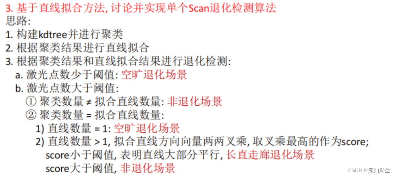
实现代码如下:
bool Icp2d::IsDegeneration()
{
if (target_cloud_->empty())
{
LOG(ERROR) << "cannot load cloud...";
return false;
}
int point_size = target_cloud_->size();
if(point_size < 500) return true; // 点数太少,空旷退化场景
LOG(INFO) << "traget_cloud size = " << point_size;
PointCloudType::Ptr target_cloud(new PointCloudType());
// 构建点云
for (size_t i = 0; i < target_scan_->ranges.size(); ++i)
{
if (target_scan_->ranges[i] < target_scan_->range_min || target_scan_->ranges[i] > target_scan_->range_max)
{
continue;
}
double real_angle = target_scan_->angle_min + i * target_scan_->angle_increment;
PointType p;
p.x = target_scan_->ranges[i] * std::cos(real_angle);
p.y = target_scan_->ranges[i] * std::sin(real_angle);
p.z = 1.0;
target_cloud->points.push_back(p);
}
pcl::search::KdTree<PointType>::Ptr kdtree; // (new pcl::search::KdTree<PointType>)
kdtree = boost::make_shared<pcl::search::KdTree<PointType>>();
// 构建kdtree
kdtree->setInputCloud(target_cloud);
pcl::EuclideanClusterExtraction<PointType> clusterExtractor;
// 创建一个向量来存储聚类的结果
std::vector<pcl::PointIndices> cluster_indices;
clusterExtractor.setClusterTolerance(0.02); // 设置聚类的距离阈值
clusterExtractor.setMinClusterSize(10); // 设置聚类的最小点数
clusterExtractor.setMaxClusterSize(1000); // 设置聚类的最大点数
clusterExtractor.setSearchMethod(kdtree); // 使用kdtree树进行加速
clusterExtractor.setInputCloud(target_cloud); // 设置点云聚类对象的输入点云数据
clusterExtractor.extract(cluster_indices); // 执行点云聚类
LOG(INFO) << "cluster size: " << cluster_indices.size();
// 创建可视化对象
pcl::visualization::PCLVisualizer viewer("Cluster Viewer");
viewer.setBackgroundColor(1.0, 1.0, 1.0);
viewer.addPointCloud<PointType>(target_cloud, "cloud");
int clusterNumber = 0; // 输出聚类结果
std::vector<Eigen::Vector3d> line_coeffs_vector;
for (const auto& indices : cluster_indices)
{
LOG(INFO) << "Cluster " << clusterNumber << " has " << indices.indices.size() << " points.";
pcl::PointCloud<PointType>::Ptr cluster(new pcl::PointCloud<PointType>);
pcl::copyPointCloud(*target_cloud, indices, *cluster);
// 拟合直线
std::vector<Eigen::Vector2d> pts;
pts.reserve(cluster->size());
for (const PointType& pt : *cluster)
{
pts.emplace_back(Eigen::Vector2d(pt.x, pt.y));
}
// 拟合直线,组装J、H和误差
Eigen::Vector3d line_coeffs;
// 利用当前点附近的几个有效近邻点,基于SVD奇异值分解,拟合出ax+by+c=0 中的最小直线系数 a,b,c,对应公式(6.11)
if (math::FitLine2D(pts, line_coeffs))
{
line_coeffs_vector.push_back(line_coeffs);
}
// 为聚类分配不同的颜色
double r = static_cast<double>(rand()) / RAND_MAX;
double g = static_cast<double>(rand()) / RAND_MAX;
double b = static_cast<double>(rand()) / RAND_MAX;
// 将聚类点云添加到可视化对象中
std::string clusterId = "cluster_" + std::to_string(clusterNumber);
viewer.addPointCloud<PointType>(cluster, clusterId);
viewer.setPointCloudRenderingProperties(pcl::visualization::PCL_VISUALIZER_COLOR, r, g, b, clusterId);
clusterNumber++;
}
int lines_size = line_coeffs_vector.size();
LOG(INFO) << "clusterNumber = " << clusterNumber << " lines_size = " << lines_size;
if(clusterNumber == lines_size)
{
if(clusterNumber == 1) return true; // 如果仅有一条直线,就是退化场景
float max_score = 0;
for(int i = 0; i < lines_size - 1; ++i)
{
for(int j = i+1; j < lines_size; ++j)
{
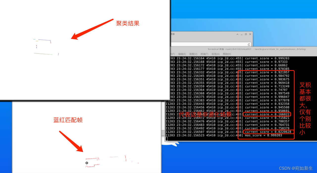
float current_score = line_coeffs_vector[i].cross(line_coeffs_vector[j]).norm();
LOG(INFO) << "current_score = " << current_score;
max_score = current_score > max_score ? current_score : max_score;
}
}
LOG(INFO) << "mas_score = " << max_score;
if(max_score < 0.3) return true; // 叉积小于阈值,代表是退化场景,直线差不多都平行
}
if (!viewer.wasStopped())
{
viewer.spinOnce(0.001);
sleep(1); //延时函数,不加的话刷新太快会看不到显示效果
viewer.close();
}
return false;
}
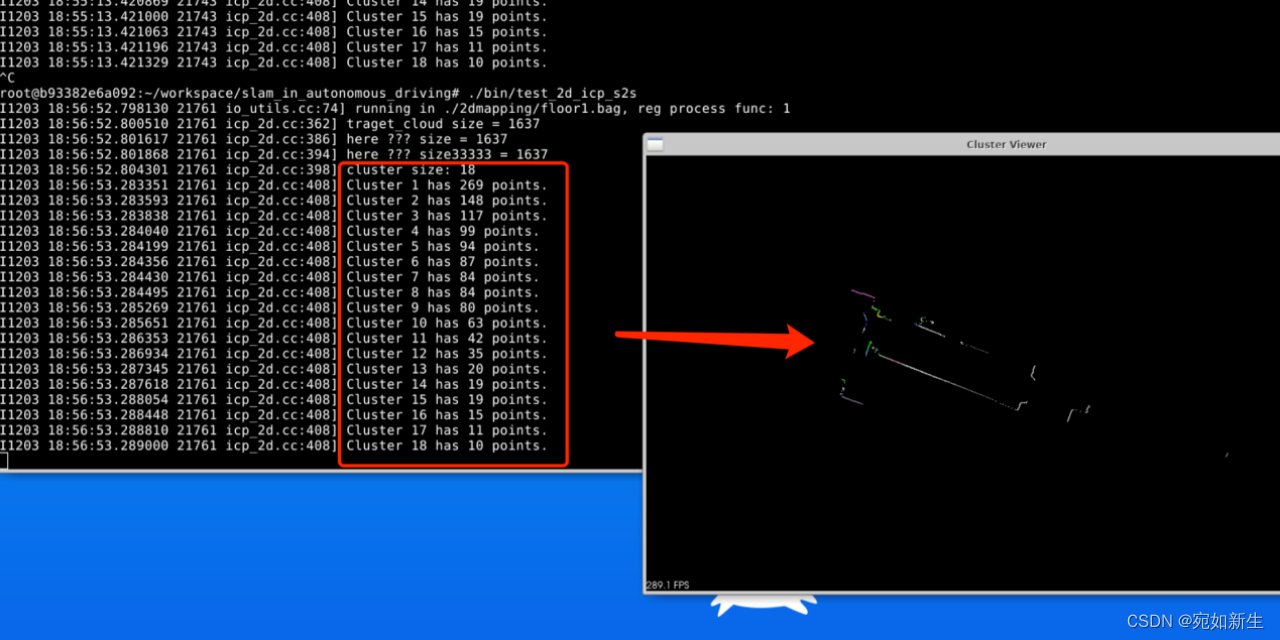
上图为聚类结果,下面是程序运行时效果。
效果展示:

4. 在诸如扫地机器人等这样基于2D激光雷达导航的机器人,如何处理悬空/低矮物体
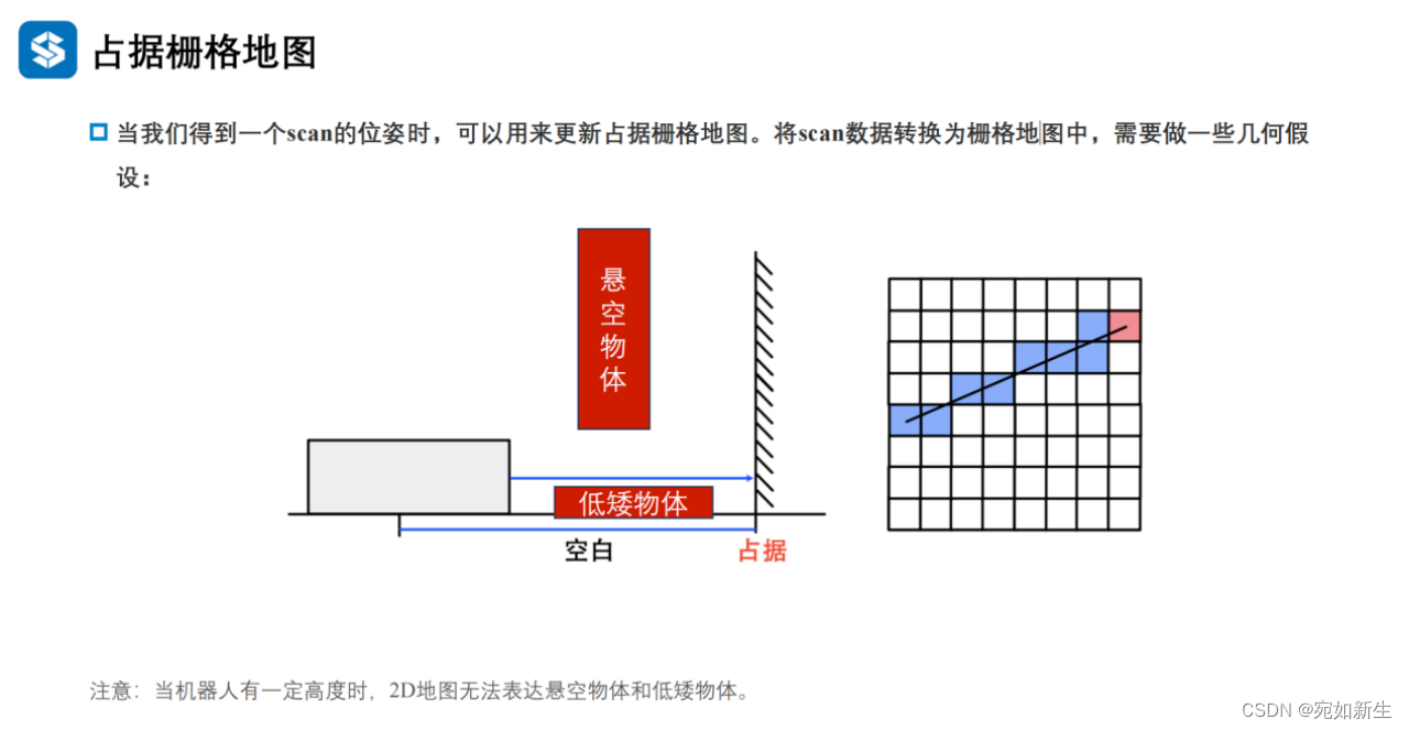
在二维SLAM方案中,如果场景中存在其他高度的障碍物或物体形状随着高度变化的情况,可以采取一些方法来处理悬空物体和低矮物体,以避免机器人与它们发生碰撞。以下是几种思路:
①可以给机器人添加三维传感器,比如RGB-D相机,将相机构建的三维地图点投影到激光雷达构建的二维栅格地图中,使得二维地图中包含高度信息。具体做法如文献[1]孙健, 刘隆辉, 李智, 杨佳玉, & 申奥. (2022). 基于rgb-d相机和激光雷达的传感器数据融合算法. 湖南工程学院学报:自然科学版, 32(1), 7.中描述的“首先将RGB-D相机获取的深度图像转换为三维点云,剔除地面点云后进行投影得到模拟2D激光数据,然后与二维激光雷达数据进行点云配准,以获取两个传感器之间的位姿关系,最后通过扩展卡尔曼滤波(EKF)将两组激光数据进行融合.实验结果表明该方法能综合利用相机和激光雷达传感器优势,有效提高机器人环境感知的完整性和建图精度. ”
②由于2D SLAM生成的占据栅格地图,是基于像素的黑白灰三色地图,我们可以人工对此地图进行“加工”,对于特定场景中存在的要躲避的三维物体预先建模,在二维栅格地图中标注出他们的位置以及高度信息,来帮助机器人更好的躲避他们。
③尝试使用普通相机对环境中的物体进行语义识别,然后把需要躲避的三维物体投影到二维平面,“告诉”机器人前面有个“物体”阻挡,不具备通过的条件。


![【MySQL语言汇总[DQL,DDL,DCL,DML]以及使用python连接数据库进行其他操作】](https://img-blog.csdnimg.cn/direct/ead04ef734e543e2a76936299d316fee.png)