文章目录
- 12.2 单目稠密 重建
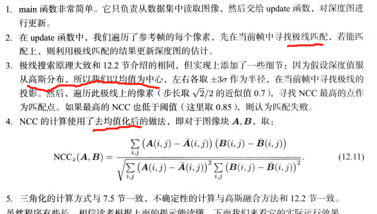
- 12.2.2 极线搜索 && 块匹配
- 12.2.3 高斯分布的深度滤波器
- 12.3 单目稠密重建 【Code】
- 待改进
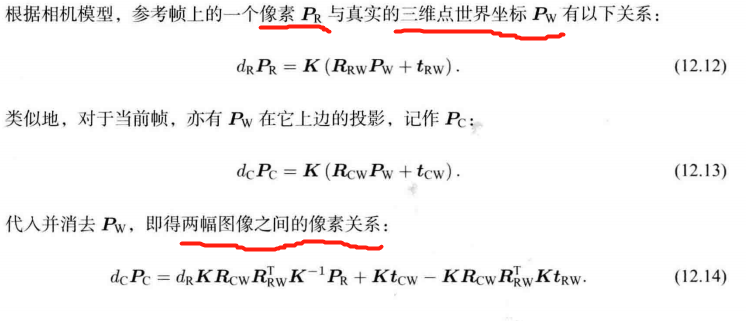
- 12.3.4 图像间的变换
- 12.4 RGB-D 稠密建图
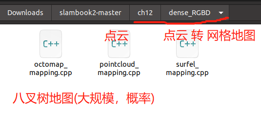
- 12.4.1 点云地图 【Code】
- 查询OpenCV版本 opencv_version
- 12.4.2 从点云 重建 网格 【Code】
- 查看PCL 版本 aptitude show libpcl-dev
- 12.4.3 八叉树地图(Octomap) 【灵活压缩、随时更新】
- 12.4.4 八叉树地图 【建模大场景】 【Code】
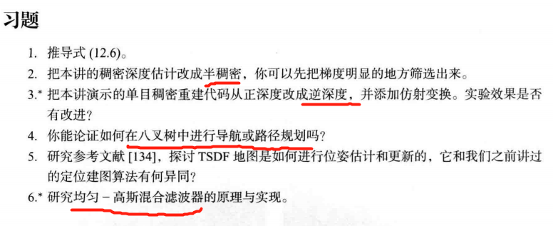
- 习题
- √ 题1
- √ 题2
- 题3
- 题4
- 题5
- 题6
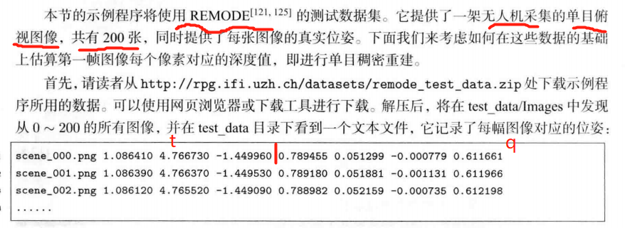
单目SLAM 稠密 深度估计
单目 稠密 重建
RGB-D 重建 的地图形式
估计 相机运动轨迹 + 特征点空间位置
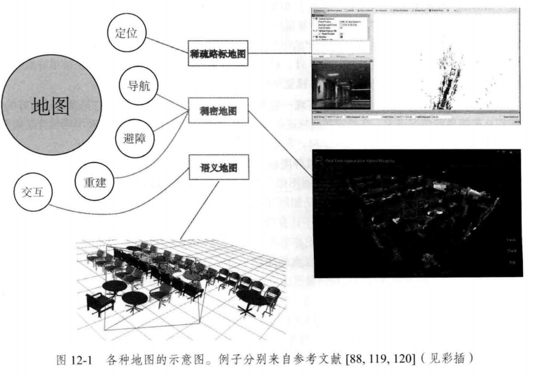
机器人SLAM:定位、导航、避障和交互
SLAM: 同时定位 与 建图
经典 SLAM 地图(路标点的集合)
视觉里程计、BA: 建模了路标点的位置
扫地机: 全局定位,导航,路径规划
增强现实设备: 将虚拟物叠加在现实物体之中, 处理虚拟物体与真实物体之间的遮挡关系。
定位(空间位姿信息): 把地图保存下来,这样只需对地图进行一次建模, 而不是每次启动机器人都重新做一次完整的SLAM
导航、避障:需要 稠密地图。哪些地方可通过
重建 三维视频通话、网上购物 纹理稠密
交互 语义地图
稀疏路标地图 只建模感兴趣部分 定位
稠密地图 建模 所有看到过的部分 导航避障
视觉SLAM 如何建 稠密地图
12.2 单目稠密 重建
获取像素点间距离的方法:
1、单目相机 三角化 计算像素之间的距离
2、双目相机, 利用左右目的视差 计算像素的距离
3、RGB-D相机 直接 获取 像素距离。
立体视觉(Stereo Vision)
移动单目相机 (移动视角的立体视觉(Moving View Stereo,MVS))
使用单目和双目 获取深度 费力不讨好。 计算量巨大、不可靠
场景: 室外,大场景
RGB-D: 量程、应用范围、光照限制。
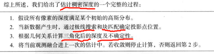
极线搜索 块匹配
深度滤波技术 :多次使用 三角测量法 让深度估计收敛。
12.2.2 极线搜索 && 块匹配
单个像素的亮度 没有区分性 ——> 比较 像素块。
计算两个小块之间的差异:
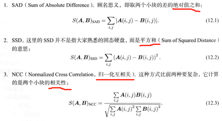
去均值 的 NCC
不断 对不同图像 进行极线 搜索时, 估计的深度分布将如何变化。
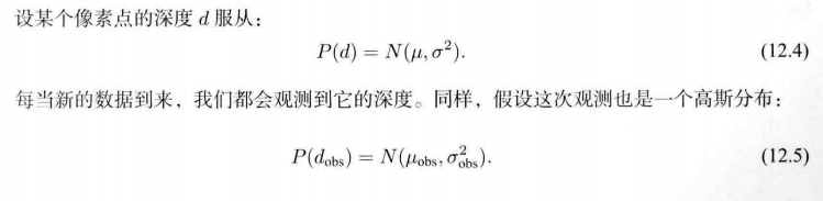
12.2.3 高斯分布的深度滤波器
均匀-高斯混合分布的滤波器
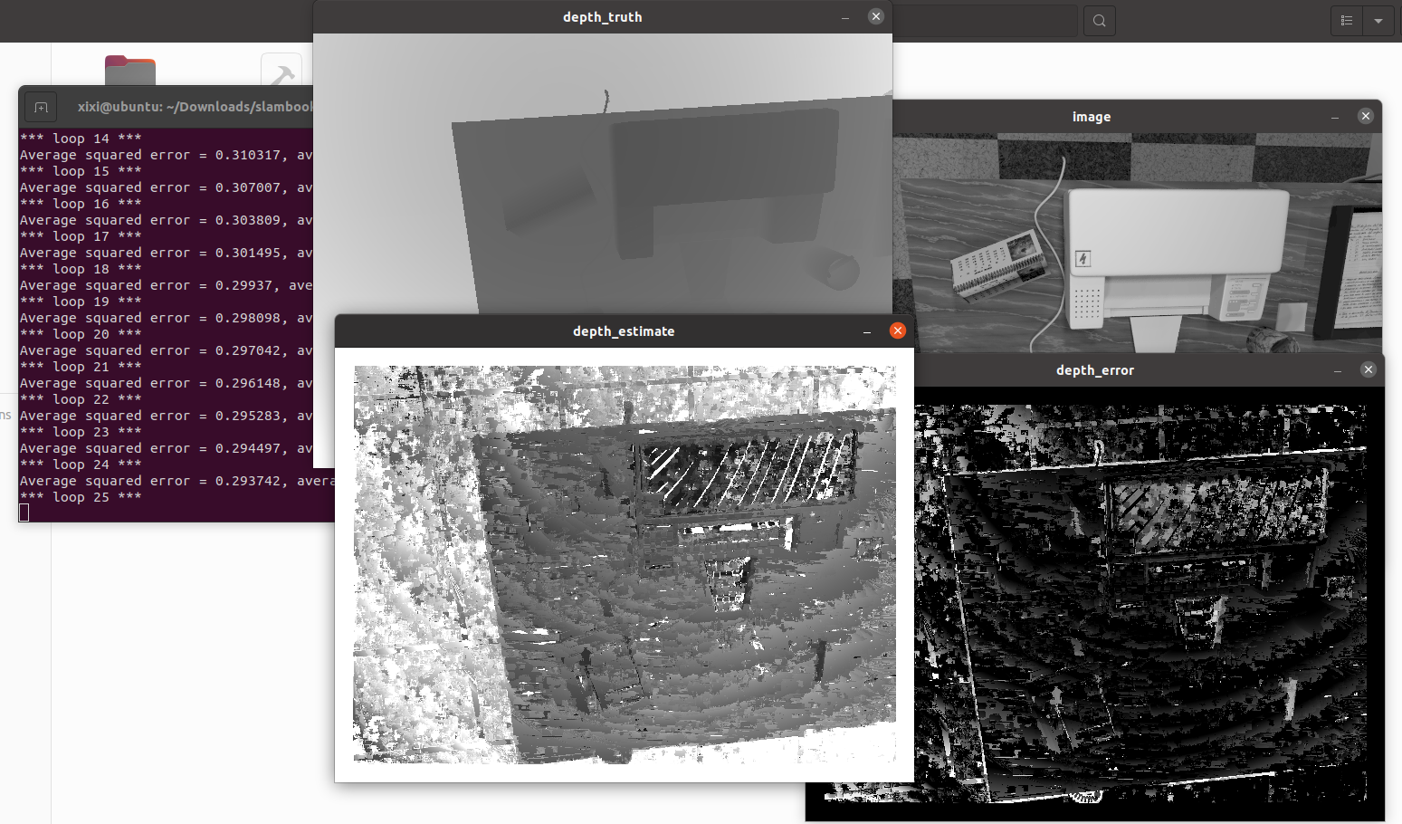
12.3 单目稠密重建 【Code】
mkdir build && cd build
cmake ..
make
./dense_mapping /home/xixi/Downloads/slambook2-master/ch12/semi_dense_mono/dataset/test_data
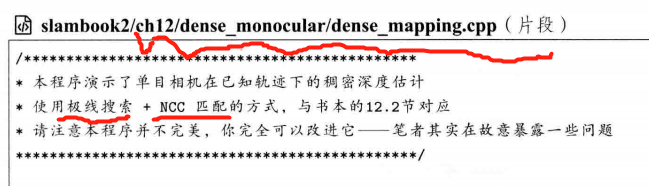
dense_mapping.cpp
#include <iostream>
#include <vector>
#include <fstream>

using namespace std;

#include <boost/timer.hpp>

// for sophus
#include <sophus/se3.h>

using Sophus::SE3; // 该文件里的全部 SE3d 都要 去掉 d

// for eigen
#include <Eigen/Core>
#include <Eigen/Geometry>

using namespace Eigen;

#include <opencv2/core/core.hpp>
#include <opencv2/highgui/highgui.hpp>
#include <opencv2/imgproc/imgproc.hpp>

using namespace cv;

/**********************************************
* 本程序演示了单目相机在已知轨迹下的稠密深度估计
* 使用极线搜索 + NCC 匹配的方式,与书本的 12.2 节对应
* 请注意本程序并不完美,你完全可以改进它——我其实在故意暴露一些问题(这是借口)。
***********************************************/

// ------------------------------------------------------------------
// parameters
const int boarder = 20;         // 边缘宽度
const int width = 640;          // 图像宽度
const int height = 480;         // 图像高度
const double fx = 481.2f;       // 相机内参
const double fy = -480.0f;
const double cx = 319.5f;
const double cy = 239.5f;
const int ncc_window_size = 3;    // NCC 取的窗口半宽度
const int ncc_area = (2 * ncc_window_size + 1) * (2 * ncc_window_size + 1); // NCC窗口面积
const double min_cov = 0.1;     // 收敛判定:最小方差
const double max_cov = 10;      // 发散判定:最大方差

// ------------------------------------------------------------------
// 重要的函数
/// 从 REMODE 数据集读取数据
bool readDatasetFiles(
    const string &path,
    vector<string> &color_image_files,
    vector<SE3> &poses,
    cv::Mat &ref_depth
);

/**
 * 根据新的图像更新深度估计
 * @param ref           参考图像
 * @param curr          当前图像
 * @param T_C_R         参考图像到当前图像的位姿
 * @param depth         深度
 * @param depth_cov     深度方差
 * @return              是否成功
 */
void update(
    const Mat &ref,
    const Mat &curr,
    const SE3 &T_C_R,
    Mat &depth,
    Mat &depth_cov2
);

/**
 * 极线搜索
 * @param ref           参考图像
 * @param curr          当前图像
 * @param T_C_R         位姿
 * @param pt_ref        参考图像中点的位置
 * @param depth_mu      深度均值
 * @param depth_cov     深度方差
 * @param pt_curr       当前点
 * @param epipolar_direction  极线方向
 * @return              是否成功
 */
bool epipolarSearch(
    const Mat &ref,
    const Mat &curr,
    const SE3 &T_C_R,
    const Vector2d &pt_ref,
    const double &depth_mu,
    const double &depth_cov,
    Vector2d &pt_curr,
    Vector2d &epipolar_direction
);

/**
 * 更新深度滤波器
 * @param pt_ref    参考图像点
 * @param pt_curr   当前图像点
 * @param T_C_R     位姿
 * @param epipolar_direction 极线方向
 * @param depth     深度均值
 * @param depth_cov2    深度方向
 * @return          是否成功
 */
bool updateDepthFilter(
    const Vector2d &pt_ref,
    const Vector2d &pt_curr,
    const SE3 &T_C_R,
    const Vector2d &epipolar_direction,
    Mat &depth,
    Mat &depth_cov2
);

/**
 * 计算 NCC 评分
 * @param ref       参考图像
 * @param curr      当前图像
 * @param pt_ref    参考点
 * @param pt_curr   当前点
 * @return          NCC评分
 */
double NCC(const Mat &ref, const Mat &curr, const Vector2d &pt_ref, const Vector2d &pt_curr);

// 双线性灰度插值
inline double getBilinearInterpolatedValue(const Mat &img, const Vector2d &pt) {
    uchar *d = &img.data[int(pt(1, 0)) * img.step + int(pt(0, 0))];
    double xx = pt(0, 0) - floor(pt(0, 0));
    double yy = pt(1, 0) - floor(pt(1, 0));
    return ((1 - xx) * (1 - yy) * double(d[0]) +
            xx * (1 - yy) * double(d[1]) +
            (1 - xx) * yy * double(d[img.step]) +
            xx * yy * double(d[img.step + 1])) / 255.0;
}

// ------------------------------------------------------------------
// 一些小工具
// 显示估计的深度图
void plotDepth(const Mat &depth_truth, const Mat &depth_estimate);

// 像素到相机坐标系
inline Vector3d px2cam(const Vector2d px) {
    return Vector3d(
        (px(0, 0) - cx) / fx,
        (px(1, 0) - cy) / fy,
        1
    );
}

// 相机坐标系到像素
inline Vector2d cam2px(const Vector3d p_cam) {
    return Vector2d(
        p_cam(0, 0) * fx / p_cam(2, 0) + cx,
        p_cam(1, 0) * fy / p_cam(2, 0) + cy
    );
}

// 检测一个点是否在图像边框内
inline bool inside(const Vector2d &pt) {
    return pt(0, 0) >= boarder && pt(1, 0) >= boarder
           && pt(0, 0) + boarder < width && pt(1, 0) + boarder <= height;
}

// 显示极线匹配
void showEpipolarMatch(const Mat &ref, const Mat &curr, const Vector2d &px_ref, const Vector2d &px_curr);

// 显示极线
void showEpipolarLine(const Mat &ref, const Mat &curr, const Vector2d &px_ref, const Vector2d &px_min_curr,
                      const Vector2d &px_max_curr);

/// 评测深度估计
void evaludateDepth(const Mat &depth_truth, const Mat &depth_estimate);
// ------------------------------------------------------------------


int main(int argc, char **argv) {
    if (argc != 2) {
        cout << "Usage: dense_mapping path_to_test_dataset" << endl;
        return -1;
    }

    // 从数据集读取数据
    vector<string> color_image_files;
    vector<SE3> poses_TWC;
    Mat ref_depth;
    bool ret = readDatasetFiles(argv[1], color_image_files, poses_TWC, ref_depth);
    if (ret == false) {
        cout << "Reading image files failed!" << endl;
        return -1;
    }
    cout << "read total " << color_image_files.size() << " files." << endl;

    // 第一张图
    Mat ref = imread(color_image_files[0], 0);                // gray-scale image
    SE3 pose_ref_TWC = poses_TWC[0];
    double init_depth = 3.0;    // 深度初始值
    double init_cov2 = 3.0;     // 方差初始值
    Mat depth(height, width, CV_64F, init_depth);             // 深度图
    Mat depth_cov2(height, width, CV_64F, init_cov2);         // 深度图方差

    for (int index = 1; index < color_image_files.size(); index++) {
        cout << "*** loop " << index << " ***" << endl;
        Mat curr = imread(color_image_files[index], 0);
        if (curr.data == nullptr) continue;
        SE3 pose_curr_TWC = poses_TWC[index];
        SE3 pose_T_C_R = pose_curr_TWC.inverse() * pose_ref_TWC;   // 坐标转换关系: T_C_W * T_W_R = T_C_R
        update(ref, curr, pose_T_C_R, depth, depth_cov2);
        evaludateDepth(ref_depth, depth);
        plotDepth(ref_depth, depth);
        imshow("image", curr);
        waitKey(1);
    }

    cout << "estimation returns, saving depth map ..." << endl;
    imwrite("depth.png", depth);
    cout << "done." << endl;

    return 0;
}

bool readDatasetFiles(
    const string &path,
    vector<string> &color_image_files,
    std::vector<SE3> &poses,
    cv::Mat &ref_depth) {
    ifstream fin(path + "/first_200_frames_traj_over_table_input_sequence.txt");
    if (!fin) return false;

    while (!fin.eof()) {
        // 数据格式:图像文件名 tx, ty, tz, qx, qy, qz, qw ,注意是 TWC 而非 TCW
        string image;
        fin >> image;
        double data[7];
        for (double &d:data) fin >> d;

        color_image_files.push_back(path + string("/images/") + image);
        poses.push_back(
            SE3(Quaterniond(data[6], data[3], data[4], data[5]),
                 Vector3d(data[0], data[1], data[2]))
        );
        if (!fin.good()) break;
    }
    fin.close();

    // load reference depth
    fin.open(path + "/depthmaps/scene_000.depth");
    ref_depth = cv::Mat(height, width, CV_64F);
    if (!fin) return false;
    for (int y = 0; y < height; y++)
        for (int x = 0; x < width; x++) {
            double depth = 0;
            fin >> depth;
            ref_depth.ptr<double>(y)[x] = depth / 100.0;
        }

    return true;
}

// 对整个深度图进行更新
void update(const Mat &ref, const Mat &curr, const SE3 &T_C_R, Mat &depth, Mat &depth_cov2) {
    for (int x = boarder; x < width - boarder; x++)
        for (int y = boarder; y < height - boarder; y++){
            // 遍历每个像素
            if (depth_cov2.ptr<double>(y)[x] < min_cov || depth_cov2.ptr<double>(y)[x] > max_cov) // 深度已收敛或发散
                continue;
            // 在极线上搜索 (x,y) 的匹配
            Vector2d pt_curr;
            Vector2d epipolar_direction;
            bool ret = epipolarSearch(
                ref,
                curr,
                T_C_R,
                Vector2d(x, y),
                depth.ptr<double>(y)[x],
                sqrt(depth_cov2.ptr<double>(y)[x]),
                pt_curr,
                epipolar_direction
            );

            if (ret == false) // 匹配失败
                continue;

            // 取消该注释以显示匹配
            // showEpipolarMatch(ref, curr, Vector2d(x, y), pt_curr);

            // 匹配成功,更新深度图
            updateDepthFilter(Vector2d(x, y), pt_curr, T_C_R, epipolar_direction, depth, depth_cov2);
        }
}

// 极线搜索
// 方法见书 12.2 12.3 两节
bool epipolarSearch(
    const Mat &ref, const Mat &curr,
    const SE3 &T_C_R, const Vector2d &pt_ref,
    const double &depth_mu, const double &depth_cov,
    Vector2d &pt_curr, Vector2d &epipolar_direction) {
    Vector3d f_ref = px2cam(pt_ref);
    f_ref.normalize();
    Vector3d P_ref = f_ref * depth_mu;    // 参考帧的 P 向量

    Vector2d px_mean_curr = cam2px(T_C_R * P_ref); // 按深度均值投影的像素
    double d_min = depth_mu - 3 * depth_cov, d_max = depth_mu + 3 * depth_cov;
    if (d_min < 0.1) d_min = 0.1;
    Vector2d px_min_curr = cam2px(T_C_R * (f_ref * d_min));    // 按最小深度投影的像素
    Vector2d px_max_curr = cam2px(T_C_R * (f_ref * d_max));    // 按最大深度投影的像素

    Vector2d epipolar_line = px_max_curr - px_min_curr;    // 极线(线段形式)
    epipolar_direction = epipolar_line;        // 极线方向
    epipolar_direction.normalize();
    double half_length = 0.5 * epipolar_line.norm();    // 极线线段的半长度
    if (half_length > 100) half_length = 100;   // 我们不希望搜索太多东西

    // 取消此句注释以显示极线(线段)
    // showEpipolarLine( ref, curr, pt_ref, px_min_curr, px_max_curr );

    // 在极线上搜索,以深度均值点为中心,左右各取半长度
    double best_ncc = -1.0;
    Vector2d best_px_curr;
    for (double l = -half_length; l <= half_length; l += 0.7) { // l+=sqrt(2)
        Vector2d px_curr = px_mean_curr + l * epipolar_direction;  // 待匹配点
        if (!inside(px_curr))
            continue;
        // 计算待匹配点与参考帧的 NCC
        double ncc = NCC(ref, curr, pt_ref, px_curr);
        if (ncc > best_ncc) {
            best_ncc = ncc;
            best_px_curr = px_curr;
        }
    }
    if (best_ncc < 0.85f)      // 只相信 NCC 很高的匹配
        return false;
    pt_curr = best_px_curr;
    return true;
}

double NCC(
    const Mat &ref, const Mat &curr,
    const Vector2d &pt_ref, const Vector2d &pt_curr) {
    // 零均值-归一化互相关
    // 先算均值
    double mean_ref = 0, mean_curr = 0;
    vector<double> values_ref, values_curr; // 参考帧和当前帧的均值
    for (int x = -ncc_window_size; x <= ncc_window_size; x++)
        for (int y = -ncc_window_size; y <= ncc_window_size; y++) {
            double value_ref = double(ref.ptr<uchar>(int(y + pt_ref(1, 0)))[int(x + pt_ref(0, 0))]) / 255.0;
            mean_ref += value_ref;

            double value_curr = getBilinearInterpolatedValue(curr, pt_curr + Vector2d(x, y));
            mean_curr += value_curr;

            values_ref.push_back(value_ref);
            values_curr.push_back(value_curr);
        }

    mean_ref /= ncc_area;
    mean_curr /= ncc_area;

    // 计算 Zero mean NCC
    double numerator = 0, demoniator1 = 0, demoniator2 = 0;
    for (int i = 0; i < values_ref.size(); i++) {
        double n = (values_ref[i] - mean_ref) * (values_curr[i] - mean_curr);
        numerator += n;
        demoniator1 += (values_ref[i] - mean_ref) * (values_ref[i] - mean_ref);
        demoniator2 += (values_curr[i] - mean_curr) * (values_curr[i] - mean_curr);
    }
    return numerator / sqrt(demoniator1 * demoniator2 + 1e-10);   // 防止分母出现零
}

bool updateDepthFilter(
    const Vector2d &pt_ref,
    const Vector2d &pt_curr,
    const SE3 &T_C_R,
    const Vector2d &epipolar_direction,
    Mat &depth,
    Mat &depth_cov2) {
    // 不知道这段还有没有人看
    // 用三角化计算深度
    SE3 T_R_C = T_C_R.inverse();
    Vector3d f_ref = px2cam(pt_ref);
    f_ref.normalize();
    Vector3d f_curr = px2cam(pt_curr);
    f_curr.normalize();

    // 方程
    // d_ref * f_ref = d_cur * ( R_RC * f_cur ) + t_RC
    // f2 = R_RC * f_cur
    // 转化成下面这个矩阵方程组
    // => [ f_ref^T f_ref, -f_ref^T f2 ] [d_ref]   [f_ref^T t]
    //    [ f_2^T f_ref, -f2^T f2      ] [d_cur] = [f2^T t   ]
    Vector3d t = T_R_C.translation();
    Vector3d f2 = T_R_C.so3() * f_curr;
    Vector2d b = Vector2d(t.dot(f_ref), t.dot(f2));
    Matrix2d A;
    A(0, 0) = f_ref.dot(f_ref);
    A(0, 1) = -f_ref.dot(f2);
    A(1, 0) = -A(0, 1);
    A(1, 1) = -f2.dot(f2);
    Vector2d ans = A.inverse() * b;
    Vector3d xm = ans[0] * f_ref;           // ref 侧的结果
    Vector3d xn = t + ans[1] * f2;          // cur 结果
    Vector3d p_esti = (xm + xn) / 2.0;      // P的位置,取两者的平均
    double depth_estimation = p_esti.norm();   // 深度值

    // 计算不确定性(以一个像素为误差)
    Vector3d p = f_ref * depth_estimation;
    Vector3d a = p - t;
    double t_norm = t.norm();
    double a_norm = a.norm();
    double alpha = acos(f_ref.dot(t) / t_norm);
    double beta = acos(-a.dot(t) / (a_norm * t_norm));
    Vector3d f_curr_prime = px2cam(pt_curr + epipolar_direction);
    f_curr_prime.normalize();
    double beta_prime = acos(f_curr_prime.dot(-t) / t_norm);
    double gamma = M_PI - alpha - beta_prime;
    double p_prime = t_norm * sin(beta_prime) / sin(gamma);
    double d_cov = p_prime - depth_estimation;
    double d_cov2 = d_cov * d_cov;

    // 高斯融合
    double mu = depth.ptr<double>(int(pt_ref(1, 0)))[int(pt_ref(0, 0))];
    double sigma2 = depth_cov2.ptr<double>(int(pt_ref(1, 0)))[int(pt_ref(0, 0))];

    double mu_fuse = (d_cov2 * mu + sigma2 * depth_estimation) / (sigma2 + d_cov2);
    double sigma_fuse2 = (sigma2 * d_cov2) / (sigma2 + d_cov2);

    depth.ptr<double>(int(pt_ref(1, 0)))[int(pt_ref(0, 0))] = mu_fuse;
    depth_cov2.ptr<double>(int(pt_ref(1, 0)))[int(pt_ref(0, 0))] = sigma_fuse2;

    return true;
}

// 后面这些太简单我就不注释了(其实是因为懒)
void plotDepth(const Mat &depth_truth, const Mat &depth_estimate) {
    imshow("depth_truth", depth_truth * 0.4);
    imshow("depth_estimate", depth_estimate * 0.4);
    imshow("depth_error", depth_truth - depth_estimate);
    waitKey(1);
}

void evaludateDepth(const Mat &depth_truth, const Mat &depth_estimate) {
    double ave_depth_error = 0;     // 平均误差
    double ave_depth_error_sq = 0;      // 平方误差
    int cnt_depth_data = 0;
    for (int y = boarder; y < depth_truth.rows - boarder; y++)
        for (int x = boarder; x < depth_truth.cols - boarder; x++) {
            double error = depth_truth.ptr<double>(y)[x] - depth_estimate.ptr<double>(y)[x];
            ave_depth_error += error;
            ave_depth_error_sq += error * error;
            cnt_depth_data++;
        }
    ave_depth_error /= cnt_depth_data;
    ave_depth_error_sq /= cnt_depth_data;

    cout << "Average squared error = " << ave_depth_error_sq << ", average error: " << ave_depth_error << endl;
}

void showEpipolarMatch(const Mat &ref, const Mat &curr, const Vector2d &px_ref, const Vector2d &px_curr) {
    Mat ref_show, curr_show;
    cv::cvtColor(ref, ref_show, COLOR_GRAY2BGR);
    cv::cvtColor(curr, curr_show, COLOR_GRAY2BGR);

    cv::circle(ref_show, cv::Point2f(px_ref(0, 0), px_ref(1, 0)), 5, cv::Scalar(0, 0, 250), 2);
    cv::circle(curr_show, cv::Point2f(px_curr(0, 0), px_curr(1, 0)), 5, cv::Scalar(0, 0, 250), 2);

    imshow("ref", ref_show);
    imshow("curr", curr_show);
    waitKey(1);
}

void showEpipolarLine(const Mat &ref, const Mat &curr, const Vector2d &px_ref, const Vector2d &px_min_curr,
                      const Vector2d &px_max_curr) {

    Mat ref_show, curr_show;
    cv::cvtColor(ref, ref_show, COLOR_GRAY2BGR);
    cv::cvtColor(curr, curr_show, COLOR_GRAY2BGR);

    cv::circle(ref_show, cv::Point2f(px_ref(0, 0), px_ref(1, 0)), 5, cv::Scalar(0, 255, 0), 2);
    cv::circle(curr_show, cv::Point2f(px_min_curr(0, 0), px_min_curr(1, 0)), 5, cv::Scalar(0, 255, 0), 2);
    cv::circle(curr_show, cv::Point2f(px_max_curr(0, 0), px_max_curr(1, 0)), 5, cv::Scalar(0, 255, 0), 2);
    cv::line(curr_show, Point2f(px_min_curr(0, 0), px_min_curr(1, 0)), Point2f(px_max_curr(0, 0), px_max_curr(1, 0)),
             Scalar(0, 255, 0), 1);

    imshow("ref", ref_show);
    imshow("curr", curr_show);
    waitKey(1);
}
CMakeLists.txt
cmake_minimum_required(VERSION 2.8)
project(dense_monocular)

set(CMAKE_CXX_STANDARD 14)

set(CMAKE_BUILD_TYPE "Debug")
set(CMAKE_CXX_FLAGS "-std=c++17 -march=native -O3")

############### dependencies ######################
# Eigen
include_directories("/usr/include/eigen3")
# OpenCV
find_package(OpenCV 4.8.0 REQUIRED)
include_directories(${OpenCV_INCLUDE_DIRS})
# Sophus
find_package(Sophus REQUIRED)
include_directories(${Sophus_INCLUDE_DIRS})

set(THIRD_PARTY_LIBS
        ${OpenCV_LIBS}
        ${Sophus_LIBRARIES})

add_executable(dense_mapping dense_mapping.cpp)
target_link_libraries(dense_mapping ${THIRD_PARTY_LIBS})
待改进
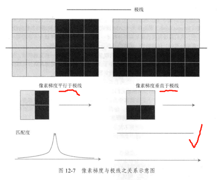
12.3.2 像素梯度
块匹配的正确与否 依赖于 图像块是否具有区分度。
立体视觉的重建质量 依赖 环境纹理。
——————————
12.3.3 逆深度(深度的倒数), 认为符合高斯分布。
12.3.4 图像间的变换
GPU 并行化 提高效率
极线搜索
其它改进:
1、给深度估计 加上 空间正则项
2、考虑错误匹配的情形: 均匀-高斯混合分布下的深度滤波器(显式地将内点与外点进行区别并进行概率建模)
————————
12.4 RGB-D 稠密建图
深度数据与纹理无关
根据估算的相机位姿,将RGB-D数据转化为点云,然后进行拼接。
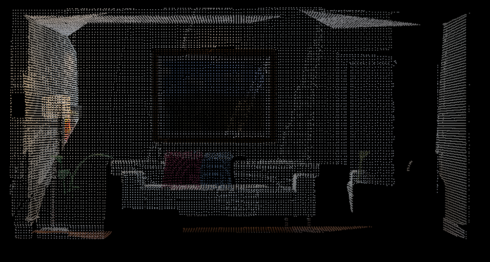
12.4.1 点云地图 【Code】
点云: 一组离散的点表示的地图。
外点去除滤波器 体素网格的降采样滤波器(Voxel grid filter)
安装点云库
sudo apt-get install libpcl-dev pcl-tools
与第5讲的变化:
1、生成每帧点云时,去掉深度值无效的点。Kinect 的量程限制
2、利用统计滤波器去除孤立点。计算附近N个点距离的平均值,去除距离均值过大的点。
3、体素网格滤波器进行降采样。
要在CMakeLists.txt文件里加这一句,使得 支持C++14标准。 可能是最新版本的PCL 要求支持C++14标准。
set(CMAKE_CXX_STANDARD 14)
查询OpenCV版本 opencv_version
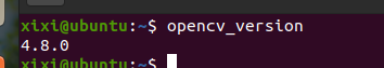
增加OpenCV的版本
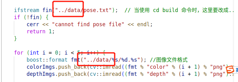
所有.cpp中的文件路径都要改成..多回一级
pointcloud_mapping.cpp
#include <iostream>
#include <fstream>

using namespace std;

#include <opencv2/core/core.hpp>
#include <opencv2/highgui/highgui.hpp>
#include <Eigen/Geometry>
#include <boost/format.hpp>  // for formating strings
#include <pcl/point_types.h>
#include <pcl/io/pcd_io.h>
#include <pcl/filters/voxel_grid.h>
#include <pcl/visualization/pcl_visualizer.h>
#include <pcl/filters/statistical_outlier_removal.h>

int main(int argc, char **argv) {
    vector<cv::Mat> colorImgs, depthImgs;    // 彩色图和深度图
    vector<Eigen::Isometry3d> poses;         // 相机位姿

    ifstream fin("../data/pose.txt");  // 当使用 cd build 命令时,这里要改成..
    if (!fin) {
        cerr << "cannot find pose file" << endl;
        return 1;
    }

    for (int i = 0; i < 5; i++) {
        boost::format fmt("../data/%s/%d.%s"); //图像文件格式
        colorImgs.push_back(cv::imread((fmt % "color" % (i + 1) % "png").str()));
        depthImgs.push_back(cv::imread((fmt % "depth" % (i + 1) % "png").str(), -1)); // 使用-1读取原始图像

        double data[7] = {0};
        for (int i = 0; i < 7; i++) {
            fin >> data[i];
        }
        Eigen::Quaterniond q(data[6], data[3], data[4], data[5]);
        Eigen::Isometry3d T(q);
        T.pretranslate(Eigen::Vector3d(data[0], data[1], data[2]));
        poses.push_back(T);
    }

    // 计算点云并拼接
    // 相机内参
    double cx = 319.5;
    double cy = 239.5;
    double fx = 481.2;
    double fy = -480.0;
    double depthScale = 5000.0;

    cout << "正在将图像转换为点云..." << endl;

    // 定义点云使用的格式:这里用的是XYZRGB
    typedef pcl::PointXYZRGB PointT;
    typedef pcl::PointCloud<PointT> PointCloud;

    // 新建一个点云
    PointCloud::Ptr pointCloud(new PointCloud);
    for (int i = 0; i < 5; i++) {
        PointCloud::Ptr current(new PointCloud);
        cout << "转换图像中: " << i + 1 << endl;
        cv::Mat color = colorImgs[i];
        cv::Mat depth = depthImgs[i];
        Eigen::Isometry3d T = poses[i];
        for (int v = 0; v < color.rows; v++)
            for (int u = 0; u < color.cols; u++) {
                unsigned int d = depth.ptr<unsigned short>(v)[u]; // 深度值
                if (d == 0) continue; // 为0表示没有测量到
                Eigen::Vector3d point;
                point[2] = double(d) / depthScale;
                point[0] = (u - cx) * point[2] / fx;
                point[1] = (v - cy) * point[2] / fy;
                Eigen::Vector3d pointWorld = T * point;

                PointT p;
                p.x = pointWorld[0];
                p.y = pointWorld[1];
                p.z = pointWorld[2];
                p.b = color.data[v * color.step + u * color.channels()];
                p.g = color.data[v * color.step + u * color.channels() + 1];
                p.r = color.data[v * color.step + u * color.channels() + 2];
                current->points.push_back(p);
            }
        // depth filter and statistical removal
        PointCloud::Ptr tmp(new PointCloud);
        pcl::StatisticalOutlierRemoval<PointT> statistical_filter;
        statistical_filter.setMeanK(50);
        statistical_filter.setStddevMulThresh(1.0);
        statistical_filter.setInputCloud(current);
        statistical_filter.filter(*tmp);
        (*pointCloud) += *tmp;
    }

    pointCloud->is_dense = false;
    cout << "点云共有" << pointCloud->size() << "个点." << endl;

    // voxel filter
    pcl::VoxelGrid<PointT> voxel_filter;
    double resolution = 0.03;
    voxel_filter.setLeafSize(resolution, resolution, resolution);       // resolution
    PointCloud::Ptr tmp(new PointCloud);
    voxel_filter.setInputCloud(pointCloud);
    voxel_filter.filter(*tmp);
    tmp->swap(*pointCloud);

    cout << "滤波之后,点云共有" << pointCloud->size() << "个点." << endl;

    pcl::io::savePCDFileBinary("map.pcd", *pointCloud);
    return 0;
}
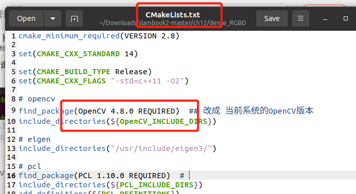
CMakeLists.txt
cmake_minimum_required(VERSION 2.8)

set(CMAKE_CXX_STANDARD 14)

set(CMAKE_BUILD_TYPE Release)
set(CMAKE_CXX_FLAGS "-std=c++11 -O2")

# opencv
find_package(OpenCV 4.8.0 REQUIRED)  ## 改成 当前系统的OpenCV版本
include_directories(${OpenCV_INCLUDE_DIRS})

# eigen
include_directories("/usr/include/eigen3/")

# pcl
find_package(PCL 1.10.0 REQUIRED)  #
include_directories(${PCL_INCLUDE_DIRS})
add_definitions(${PCL_DEFINITIONS})

# octomap
find_package(octomap REQUIRED)
include_directories(${OCTOMAP_INCLUDE_DIRS})

add_executable(pointcloud_mapping pointcloud_mapping.cpp)
target_link_libraries(pointcloud_mapping ${OpenCV_LIBS} ${PCL_LIBRARIES})

add_executable(octomap_mapping octomap_mapping.cpp)
target_link_libraries(octomap_mapping ${OpenCV_LIBS} ${PCL_LIBRARIES} ${OCTOMAP_LIBRARIES})

add_executable(surfel_mapping surfel_mapping.cpp)
target_link_libraries(surfel_mapping ${OpenCV_LIBS} ${PCL_LIBRARIES})
mkdir build && cd build   ## 需要将.cpp中数据的路径 多加一个.
cmake ..
make
./pointcloud_mapping
pcl_viewer map.pcd
体素滤波之后的点云:
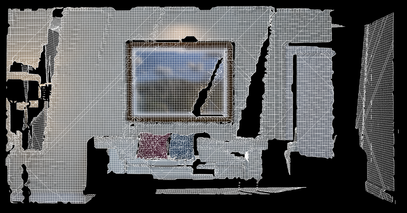
12.4.2 从点云 重建 网格 【Code】
./surfel_mapping map.pcd
点云转换成 网格地图(栅格地图)。
surfel_mapping.cpp
//
// Created by gaoxiang on 19-4-25.
//

#include <pcl/point_cloud.h>
#include <pcl/point_types.h>
#include <pcl/io/pcd_io.h>
#include <pcl/visualization/pcl_visualizer.h>
#include <pcl/kdtree/kdtree_flann.h>
#include <pcl/surface/surfel_smoothing.h>
#include <pcl/surface/mls.h>
#include <pcl/surface/gp3.h>
#include <pcl/surface/impl/mls.hpp>

// typedefs
typedef pcl::PointXYZRGB PointT;
typedef pcl::PointCloud<PointT> PointCloud;
typedef pcl::PointCloud<PointT>::Ptr PointCloudPtr;
typedef pcl::PointXYZRGBNormal SurfelT;
typedef pcl::PointCloud<SurfelT> SurfelCloud;
typedef pcl::PointCloud<SurfelT>::Ptr SurfelCloudPtr;

SurfelCloudPtr reconstructSurface(
        const PointCloudPtr &input, float radius, int polynomial_order) {
    pcl::MovingLeastSquares<PointT, SurfelT> mls;
    pcl::search::KdTree<PointT>::Ptr tree(new pcl::search::KdTree<PointT>);
    mls.setSearchMethod(tree);
    mls.setSearchRadius(radius);
    mls.setComputeNormals(true);
    mls.setSqrGaussParam(radius * radius);
    mls.setPolynomialFit(polynomial_order > 1);
    mls.setPolynomialOrder(polynomial_order);
    mls.setInputCloud(input);
    SurfelCloudPtr output(new SurfelCloud);
    mls.process(*output);
    return (output);
}

pcl::PolygonMeshPtr triangulateMesh(const SurfelCloudPtr &surfels) {
    // Create search tree*
    pcl::search::KdTree<SurfelT>::Ptr tree(new pcl::search::KdTree<SurfelT>);
    tree->setInputCloud(surfels);

    // Initialize objects
    pcl::GreedyProjectionTriangulation<SurfelT> gp3;
    pcl::PolygonMeshPtr triangles(new pcl::PolygonMesh);

    // Set the maximum distance between connected points (maximum edge length)
    gp3.setSearchRadius(0.05);

    // Set typical values for the parameters
    gp3.setMu(2.5);
    gp3.setMaximumNearestNeighbors(100);
    gp3.setMaximumSurfaceAngle(M_PI / 4); // 45 degrees
    gp3.setMinimumAngle(M_PI / 18); // 10 degrees
    gp3.setMaximumAngle(2 * M_PI / 3); // 120 degrees
    gp3.setNormalConsistency(true);

    // Get result
    gp3.setInputCloud(surfels);
    gp3.setSearchMethod(tree);
    gp3.reconstruct(*triangles);

    return triangles;
}

int main(int argc, char **argv) {

    // Load the points
    PointCloudPtr cloud(new PointCloud);
    if (argc == 0 || pcl::io::loadPCDFile(argv[1], *cloud)) {
        cout << "failed to load point cloud!";
        return 1;
    }
    cout << "point cloud loaded, points: " << cloud->points.size() << endl;

    // Compute surface elements
    cout << "computing normals ... " << endl;
    double mls_radius = 0.05, polynomial_order = 2;
    auto surfels = reconstructSurface(cloud, mls_radius, polynomial_order);

    // Compute a greedy surface triangulation
    cout << "computing mesh ... " << endl;
    pcl::PolygonMeshPtr mesh = triangulateMesh(surfels);

    cout << "display mesh ... " << endl;
    pcl::visualization::PCLVisualizer vis;
    vis.addPolylineFromPolygonMesh(*mesh, "mesh frame");
    vis.addPolygonMesh(*mesh, "mesh");
    vis.resetCamera();
    vis.spin();
}
重建算法: Moving Least Square 、 Greedy Projection
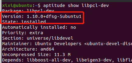
查看PCL 版本 aptitude show libpcl-dev
aptitude show libpcl-dev
可参考链接
12.4.3 八叉树地图(Octomap) 【灵活压缩、随时更新】
点云地图 不足:
1、占内存,提供了很多不必要的细节
2、无法处理运动物体。 只有 “添加点”,点消失时 不会 被移除。
八叉树 比 点云 节省大量的存储空间
- 当某个方块的所有子结点都被占据或都不被占据时,就没必要展开。
12.4.4 八叉树地图 【建模大场景】 【Code】
安装 octomap库
sudo apt-get install liboctomap-dev octovis
./octomap_mapping
octovis octomap.bt
动图截取:
byzanz-record -x 72 -y 64 -w 1848 -h 893 -d 10 --delay=5 -c /home/xixi/myGIF/test.gif

octomap_mapping.cpp
#include <iostream>
#include <fstream>

using namespace std;

#include <opencv2/core/core.hpp>
#include <opencv2/highgui/highgui.hpp>

#include <octomap/octomap.h>    // for octomap

#include <Eigen/Geometry>
#include <boost/format.hpp>  // for formating strings

int main(int argc, char **argv) {
    vector<cv::Mat> colorImgs, depthImgs;    // 彩色图和深度图
    vector<Eigen::Isometry3d> poses;         // 相机位姿

    ifstream fin("../data/pose.txt");
    if (!fin) {
        cerr << "cannot find pose file" << endl;
        return 1;
    }

    for (int i = 0; i < 5; i++) {
        boost::format fmt("../data/%s/%d.%s"); //图像文件格式
        colorImgs.push_back(cv::imread((fmt % "color" % (i + 1) % "png").str()));
        depthImgs.push_back(cv::imread((fmt % "depth" % (i + 1) % "png").str(), -1)); // 使用-1读取原始图像

        double data[7] = {0};
        for (int i = 0; i < 7; i++) {
            fin >> data[i];
        }
        Eigen::Quaterniond q(data[6], data[3], data[4], data[5]);
        Eigen::Isometry3d T(q);
        T.pretranslate(Eigen::Vector3d(data[0], data[1], data[2]));
        poses.push_back(T);
    }

    // 计算点云并拼接
    // 相机内参
    double cx = 319.5;
    double cy = 239.5;
    double fx = 481.2;
    double fy = -480.0;
    double depthScale = 5000.0;

    cout << "正在将图像转换为 Octomap ..." << endl;

    // octomap tree
    octomap::OcTree tree(0.01); // 参数为分辨率

    for (int i = 0; i < 5; i++) {
        cout << "转换图像中: " << i + 1 << endl;
        cv::Mat color = colorImgs[i];
        cv::Mat depth = depthImgs[i];
        Eigen::Isometry3d T = poses[i];

        octomap::Pointcloud cloud;  // the point cloud in octomap

        for (int v = 0; v < color.rows; v++)
            for (int u = 0; u < color.cols; u++) {
                unsigned int d = depth.ptr<unsigned short>(v)[u]; // 深度值
                if (d == 0) continue; // 为0表示没有测量到
                Eigen::Vector3d point;
                point[2] = double(d) / depthScale;
                point[0] = (u - cx) * point[2] / fx;
                point[1] = (v - cy) * point[2] / fy;
                Eigen::Vector3d pointWorld = T * point;
                // 将世界坐标系的点放入点云
                cloud.push_back(pointWorld[0], pointWorld[1], pointWorld[2]);
            }

        // 将点云存入八叉树地图,给定原点,这样可以计算投射线
        tree.insertPointCloud(cloud, octomap::point3d(T(0, 3), T(1, 3), T(2, 3)));
    }

    // 更新中间节点的占据信息并写入磁盘
    tree.updateInnerOccupancy();
    cout << "saving octomap ... " << endl;
    tree.writeBinary("octomap.bt");
    return 0;
}
——————————
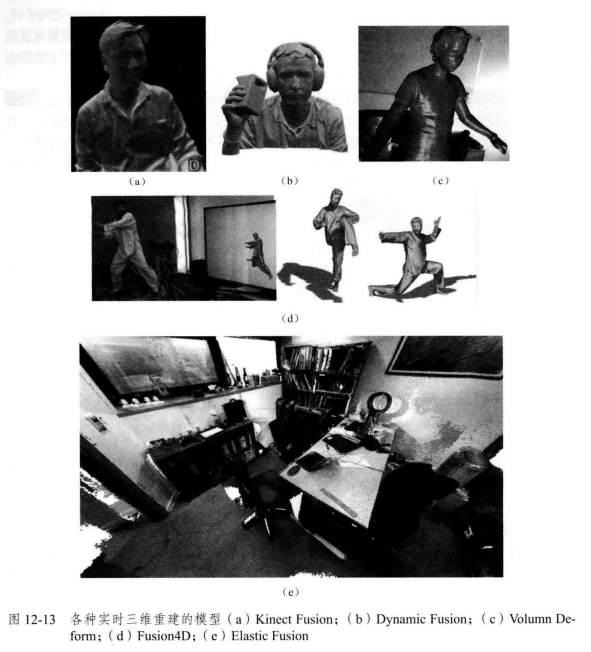
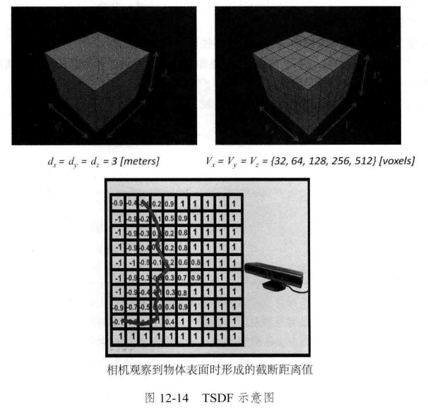
12.5 TSDF 地图 和 Fusion系列
TSDF(Truncated Signed Distance Function,截断符号距离函数)
实时三维重建: 重建准确地图
定位算法 可以满足实时性需求,地图加工可在关键帧处进行处理,无需实时。
SLAM 轻量级、小型化
实时三维重建 大规模、大型动态场景。
——————————
12.6 小结
度量地图
RGB-D 构建稠密地图 更容易、更稳定一些
习题
√ 题1

#*********************************解题1开始
设某个像素点的深度
d
d
d 服从高斯分布
P
(
d
)
=
N
(
μ
,
σ
2
)
P(d) = N(\mu, σ^2)
P(d)=N(μ,σ2)
增加新数据后,重新观测到的深度分布符合高斯分布 P ( d o b s ) = N ( μ o b s , σ o b s 2 ) P(d_{obs}) = N(\mu_{obs}, σ_{obs}^2) P(dobs)=N(μobs,σobs2)
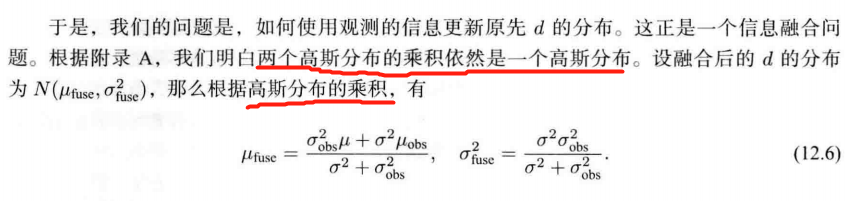
信息融合后的深度为这两个高斯分布的乘积,即
P
(
d
f
u
s
e
)
=
N
(
μ
,
σ
2
)
⋅
N
(
μ
o
b
s
,
σ
o
b
s
2
)
=
1
2
π
σ
e
x
p
(
−
1
2
(
x
−
μ
)
2
σ
2
)
⋅
1
2
π
σ
o
b
s
e
x
p
(
−
1
2
(
x
−
μ
o
b
s
)
2
σ
o
b
s
2
)
=
1
2
π
σ
σ
o
b
s
e
x
p
(
−
1
2
(
x
−
μ
)
2
σ
2
−
1
2
(
x
−
μ
o
b
s
)
2
σ
o
b
s
2
)
=
1
2
π
σ
σ
o
b
s
e
x
p
(
−
1
2
σ
o
b
s
2
⋅
(
x
−
μ
)
2
+
σ
2
⋅
(
x
−
μ
o
b
s
)
2
σ
2
σ
o
b
s
2
)
=
1
2
π
σ
σ
o
b
s
e
x
p
(
−
1
2
(
σ
o
b
s
2
+
σ
2
)
⋅
x
2
−
2
(
σ
o
b
s
2
μ
+
σ
2
μ
o
b
s
)
⋅
x
+
σ
o
b
s
2
μ
2
+
σ
2
μ
o
b
s
2
σ
2
σ
o
b
s
2
)
=
1
2
π
σ
σ
o
b
s
e
x
p
(
−
1
2
x
2
−
2
σ
o
b
s
2
μ
+
σ
2
μ
o
b
s
σ
o
b
s
2
+
σ
2
⋅
x
+
σ
o
b
s
2
μ
2
+
σ
2
μ
o
b
s
2
σ
o
b
s
2
+
σ
2
σ
2
σ
o
b
s
2
σ
o
b
s
2
+
σ
2
)
=
1
2
π
σ
σ
o
b
s
e
x
p
(
−
1
2
(
x
−
σ
o
b
s
2
μ
+
σ
2
μ
o
b
s
σ
o
b
s
2
+
σ
2
)
2
σ
2
σ
o
b
s
2
σ
o
b
s
2
+
σ
2
)
⋅
e
x
p
(
−
1
2
σ
o
b
s
2
μ
2
+
σ
2
μ
o
b
s
2
σ
o
b
s
2
+
σ
2
−
(
σ
o
b
s
2
μ
+
σ
2
μ
o
b
s
σ
o
b
s
2
+
σ
2
)
2
σ
2
σ
o
b
s
2
σ
o
b
s
2
+
σ
2
)
=
1
2
π
σ
σ
o
b
s
σ
o
b
s
2
+
σ
2
e
x
p
(
−
1
2
(
x
−
σ
o
b
s
2
μ
+
σ
2
μ
o
b
s
σ
o
b
s
2
+
σ
2
)
2
σ
2
σ
o
b
s
2
σ
o
b
s
2
+
σ
2
)
⋅
e
x
p
(
−
1
2
σ
o
b
s
2
μ
2
+
σ
2
μ
o
b
s
2
σ
o
b
s
2
+
σ
2
−
(
σ
o
b
s
2
μ
+
σ
2
μ
o
b
s
σ
o
b
s
2
+
σ
2
)
2
σ
2
σ
o
b
s
2
σ
o
b
s
2
+
σ
2
)
2
π
σ
o
b
s
2
+
σ
2
\begin{align*}P(d_{fuse}) &= N(\mu, σ^2) ·N(\mu_{obs}, σ_{obs}^2) \\ & = \frac{1}{\sqrt{2\pi}\sigma}exp(-\frac{1}{2}\frac{(x-\mu)^2}{\sigma^2}) · \frac{1}{\sqrt{2\pi}\sigma_{obs}}exp(-\frac{1}{2}\frac{(x-\mu_{obs})^2}{\sigma_{obs}^2}) \\ &= \frac{1}{2\pi\sigma\sigma_{obs}}exp(-\frac{1}{2}\frac{(x-\mu)^2}{\sigma^2}-\frac{1}{2}\frac{(x-\mu_{obs})^2}{\sigma_{obs}^2})\\ &= \frac{1}{2\pi\sigma\sigma_{obs}}exp(-\frac{1}{2}\frac{\sigma_{obs}^2·(x-\mu)^2+\sigma^2·(x-\mu_{obs})^2}{\sigma^2\sigma_{obs}^2})\\ &= \frac{1}{2\pi\sigma\sigma_{obs}}exp(-\frac{1}{2}\frac{(\sigma_{obs}^2+\sigma^2)·x^2-2(\sigma_{obs}^2\mu+\sigma^2\mu_{obs})·x+\sigma_{obs}^2\mu^2+\sigma^2\mu_{obs}^2}{\sigma^2\sigma_{obs}^2})\\ &= \frac{1}{2\pi\sigma\sigma_{obs}}exp(-\frac{1}{2}\frac{x^2-2\frac{\sigma_{obs}^2\mu+\sigma^2\mu_{obs}}{\sigma_{obs}^2+\sigma^2}·x+\frac{\sigma_{obs}^2\mu^2+\sigma^2\mu_{obs}^2}{\sigma_{obs}^2+\sigma^2}}{\frac{\sigma^2\sigma_{obs}^2}{\sigma_{obs}^2+\sigma^2}})\\ &= \frac{1}{2\pi\sigma\sigma_{obs}}exp(-\frac{1}{2}\frac{(x-\frac{\sigma_{obs}^2\mu+\sigma^2\mu_{obs}}{\sigma_{obs}^2+\sigma^2})^2}{\frac{\sigma^2\sigma_{obs}^2}{\sigma_{obs}^2+\sigma^2}})·exp(-\frac{1}{2}\frac{\frac{\sigma_{obs}^2\mu^2+\sigma^2\mu_{obs}^2}{\sigma_{obs}^2+\sigma^2}-(\frac{\sigma_{obs}^2\mu+\sigma^2\mu_{obs}}{\sigma_{obs}^2+\sigma^2})^2}{\frac{\sigma^2\sigma_{obs}^2}{\sigma_{obs}^2+\sigma^2}})\\ &= \frac{1}{\sqrt{2\pi}\frac{\sigma\sigma_{obs}}{\sqrt{\sigma_{obs}^2+\sigma^2}}}exp(-\frac{1}{2}\frac{(x-\frac{\sigma_{obs}^2\mu+\sigma^2\mu_{obs}}{\sigma_{obs}^2+\sigma^2})^2}{\frac{\sigma^2\sigma_{obs}^2}{\sigma_{obs}^2+\sigma^2}})·\frac{exp(-\frac{1}{2}\frac{\frac{\sigma_{obs}^2\mu^2+\sigma^2\mu_{obs}^2}{\sigma_{obs}^2+\sigma^2}-(\frac{\sigma_{obs}^2\mu+\sigma^2\mu_{obs}}{\sigma_{obs}^2+\sigma^2})^2}{\frac{\sigma^2\sigma_{obs}^2}{\sigma_{obs}^2+\sigma^2}})}{\sqrt{2\pi}\sqrt{\sigma_{obs}^2+\sigma^2}}\\ \end{align*}
P(dfuse)=N(μ,σ2)⋅N(μobs,σobs2)=2πσ1exp(−21σ2(x−μ)2)⋅2πσobs1exp(−21σobs2(x−μobs)2)=2πσσobs1exp(−21σ2(x−μ)2−21σobs2(x−μobs)2)=2πσσobs1exp(−21σ2σobs2σobs2⋅(x−μ)2+σ2⋅(x−μobs)2)=2πσσobs1exp(−21σ2σobs2(σobs2+σ2)⋅x2−2(σobs2μ+σ2μobs)⋅x+σobs2μ2+σ2μobs2)=2πσσobs1exp(−21σobs2+σ2σ2σobs2x2−2σobs2+σ2σobs2μ+σ2μobs⋅x+σobs2+σ2σobs2μ2+σ2μobs2)=2πσσobs1exp(−21σobs2+σ2σ2σobs2(x−σobs2+σ2σobs2μ+σ2μobs)2)⋅exp(−21σobs2+σ2σ2σobs2σobs2+σ2σobs2μ2+σ2μobs2−(σobs2+σ2σobs2μ+σ2μobs)2)=2πσobs2+σ2σσobs1exp(−21σobs2+σ2σ2σobs2(x−σobs2+σ2σobs2μ+σ2μobs)2)⋅2πσobs2+σ2exp(−21σobs2+σ2σ2σobs2σobs2+σ2σobs2μ2+σ2μobs2−(σobs2+σ2σobs2μ+σ2μobs)2)
显然,前面部分符合高斯分布
N
(
μ
f
u
s
e
,
σ
f
u
s
e
2
)
N(\mu_{fuse}, σ_{fuse}^2)
N(μfuse,σfuse2),其中
μ
f
u
s
e
=
σ
o
b
s
2
μ
+
σ
2
μ
o
b
s
σ
o
b
s
2
+
σ
2
,
,
,
σ
f
u
s
e
2
=
σ
2
σ
o
b
s
2
σ
o
b
s
2
+
σ
2
\mu_{fuse} = \frac{\sigma_{obs}^2\mu+\sigma^2\mu_{obs}}{\sigma_{obs}^2+\sigma^2}, ,, σ_{fuse}^2=\frac{\sigma^2\sigma_{obs}^2}{\sigma_{obs}^2+\sigma^2}
μfuse=σobs2+σ2σobs2μ+σ2μobs,,,σfuse2=σobs2+σ2σ2σobs2
后面部分为 常数,不影响其高斯分布类型
关于这个常数的补充说明如下,供参考
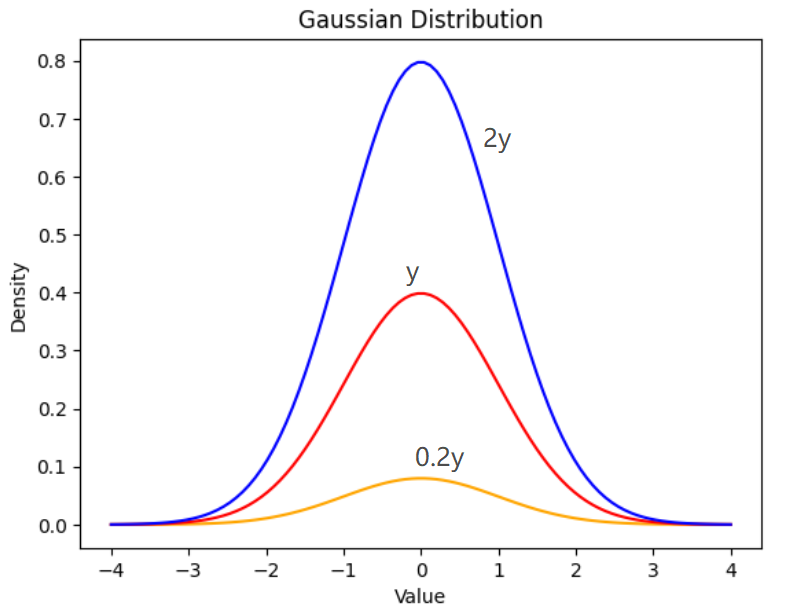
import numpy as np
import matplotlib.pyplot as plt

# 绘制高斯分布曲线
x = np.linspace(-4, 4, 100)
y = gaussian.pdf(x)

plt.plot(x, 0.2*y, 'orange')
plt.plot(x, y, 'r')
plt.plot(x, 2*y, 'b')

plt.xlabel('Value')
plt.ylabel('Density')
plt.title('Gaussian Distribution')

plt.show()
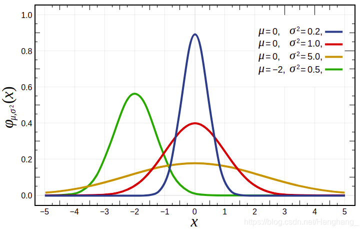
正态分布的数学期望值或期望值
μ
μ
μ 等于位置参数,决定了分布的位置;其方差
σ
2
\sigma ^{2}
σ2 等于尺度参数,决定了分布的幅度。
#*********************************解题1结束
√ 题2
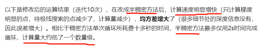
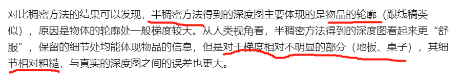
半稠密深度估计,先把梯度明显的地方筛选出来。
数据集下载链接: https://rpg.ifi.uzh.ch/datasets/remode_test_data.zip
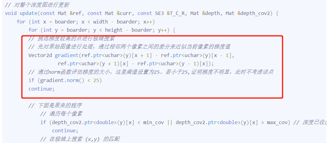
在 update 函数部分添加梯度比较和筛选代码。
#*********************************解题2开始
建 空白文件
touch CMakeLists.txt
touch semi_dense_mapping.cpp
复制相应的代码
报错:
/home/xixi/Downloads/slambook2-master/ch12/dense_mono/dense_mapping.cpp:12:15: error: ‘Sophus::SE3d’ has not been declared
12 | using Sophus::SE3d;
解决办法链接
报错原因:没将 update函数的类型改为 void
mkdir build && cd build
cmake ..
make
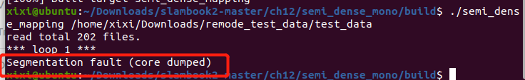
./semi_dense_mapping /home/xixi/Downloads/slambook2-master/ch12/semi_dense_mono/dataset/test_data

CMakeLists.txt
cmake_minimum_required(VERSION 2.8)
project(semi_dense_monocular)

set(CMAKE_BUILD_TYPE "Release")
set(CMAKE_CXX_FLAGS "-std=c++11 -march=native -O3")

############### dependencies ######################
# Eigen
include_directories("/usr/include/eigen3")
# OpenCV
find_package(OpenCV 4 REQUIRED)  ## OpenCV是4.8.0 .cpp文件需要修改
include_directories(${OpenCV_INCLUDE_DIRS})
# Sophus
find_package(Sophus REQUIRED)
include_directories(${Sophus_INCLUDE_DIRS})

set(THIRD_PARTY_LIBS
        ${OpenCV_LIBS}
        ${Sophus_LIBRARIES})

add_executable(semi_dense_mapping semi_dense_mapping.cpp)
target_link_libraries(semi_dense_mapping ${THIRD_PARTY_LIBS})
semi_dense_mapping.cpp
#include <iostream>
#include <vector>
#include <fstream>
#include <chrono>

using namespace std;

#include <boost/timer.hpp>

// for sophus
#include <sophus/se3.h> // 修改

using Sophus::SE3; // 修改  本代码里的 SE3d 的 d 都要去掉

// for eigen
#include <Eigen/Core>
#include <Eigen/Geometry>

using namespace Eigen;

#include <opencv2/core/core.hpp>
#include <opencv2/highgui/highgui.hpp>
#include <opencv2/imgproc/imgproc.hpp>

using namespace cv;

/**********************************************
* 本程序演示了单目相机在已知轨迹下的稠密深度估计
* 使用极线搜索 + NCC 匹配的方式,与书本的 12.2 节对应
* 请注意本程序并不完美,你完全可以改进它——我其实在故意暴露一些问题(这是借口)。
***********************************************/

// ------------------------------------------------------------------
// parameters
const int boarder = 20;         // 边缘宽度
const int width = 640;          // 图像宽度
const int height = 480;         // 图像高度
const double fx = 481.2f;       // 相机内参
const double fy = -480.0f;
const double cx = 319.5f;
const double cy = 239.5f;
const int ncc_window_size = 3;    // NCC 取的窗口半宽度
const int ncc_area = (2 * ncc_window_size + 1) * (2 * ncc_window_size + 1); // NCC窗口面积
const double min_cov = 0.1;     // 收敛判定:最小方差
const double max_cov = 10;      // 发散判定:最大方差

// ------------------------------------------------------------------
// 重要的函数
/// 从 REMODE 数据集读取数据
bool readDatasetFiles(
    const string &path,
    vector<string> &color_image_files,
    vector<SE3> &poses,
    cv::Mat &ref_depth
);

/**
 * 根据新的图像更新深度估计
 * @param ref           参考图像
 * @param curr          当前图像
 * @param T_C_R         参考图像到当前图像的位姿
 * @param depth         深度
 * @param depth_cov     深度方差
 * @return              是否成功
 */
void update(
    const Mat &ref,
    const Mat &curr,
    const SE3 &T_C_R,
    Mat &depth,
    Mat &depth_cov2
);

/**
 * 极线搜索
 * @param ref           参考图像
 * @param curr          当前图像
 * @param T_C_R         位姿
 * @param pt_ref        参考图像中点的位置
 * @param depth_mu      深度均值
 * @param depth_cov     深度方差
 * @param pt_curr       当前点
 * @param epipolar_direction  极线方向
 * @return              是否成功
 */
bool epipolarSearch(
    const Mat &ref,
    const Mat &curr,
    const SE3 &T_C_R,
    const Vector2d &pt_ref,
    const double &depth_mu,
    const double &depth_cov,
    Vector2d &pt_curr,
    Vector2d &epipolar_direction
);

/**
 * 更新深度滤波器
 * @param pt_ref    参考图像点
 * @param pt_curr   当前图像点
 * @param T_C_R     位姿
 * @param epipolar_direction 极线方向
 * @param depth     深度均值
 * @param depth_cov2    深度方向
 * @return          是否成功
 */
bool updateDepthFilter(
    const Vector2d &pt_ref,
    const Vector2d &pt_curr,
    const SE3 &T_C_R,
    const Vector2d &epipolar_direction,
    Mat &depth,
    Mat &depth_cov2
);

/**
 * 计算 NCC 评分
 * @param ref       参考图像
 * @param curr      当前图像
 * @param pt_ref    参考点
 * @param pt_curr   当前点
 * @return          NCC评分
 */
double NCC(const Mat &ref, const Mat &curr, const Vector2d &pt_ref, const Vector2d &pt_curr);

// 双线性灰度插值
inline double getBilinearInterpolatedValue(const Mat &img, const Vector2d &pt) {
    uchar *d = &img.data[int(pt(1, 0)) * img.step + int(pt(0, 0))];
    double xx = pt(0, 0) - floor(pt(0, 0));
    double yy = pt(1, 0) - floor(pt(1, 0));
    return ((1 - xx) * (1 - yy) * double(d[0]) +
            xx * (1 - yy) * double(d[1]) +
            (1 - xx) * yy * double(d[img.step]) +
            xx * yy * double(d[img.step + 1])) / 255.0;
}

// ------------------------------------------------------------------
// 一些小工具
// 显示估计的深度图
void plotDepth(const Mat &depth_truth, const Mat &depth_estimate);

// 像素到相机坐标系
inline Vector3d px2cam(const Vector2d px) {
    return Vector3d(
        (px(0, 0) - cx) / fx,
        (px(1, 0) - cy) / fy,
        1
    );
}

// 相机坐标系到像素
inline Vector2d cam2px(const Vector3d p_cam) {
    return Vector2d(
        p_cam(0, 0) * fx / p_cam(2, 0) + cx,
        p_cam(1, 0) * fy / p_cam(2, 0) + cy
    );
}

// 检测一个点是否在图像边框内
inline bool inside(const Vector2d &pt) {
    return pt(0, 0) >= boarder && pt(1, 0) >= boarder
           && pt(0, 0) + boarder < width && pt(1, 0) + boarder <= height;
}

// 显示极线匹配
void showEpipolarMatch(const Mat &ref, const Mat &curr, const Vector2d &px_ref, const Vector2d &px_curr);

// 显示极线
void showEpipolarLine(const Mat &ref, const Mat &curr, const Vector2d &px_ref, const Vector2d &px_min_curr,
                      const Vector2d &px_max_curr);

/// 评测深度估计
void evaludateDepth(const Mat &depth_truth, const Mat &depth_estimate);
// ------------------------------------------------------------------


int main(int argc, char **argv) {
    if (argc != 2) {
        cout << "Usage: dense_mapping path_to_test_dataset" << endl;
        return -1;
    }

    // 从数据集读取数据
    vector<string> color_image_files;
    vector<SE3> poses_TWC;
    Mat ref_depth;
    bool ret = readDatasetFiles(argv[1], color_image_files, poses_TWC, ref_depth);
    if (ret == false) {
        cout << "Reading image files failed!" << endl;
        return -1;
    }
    cout << "read total " << color_image_files.size() << " files." << endl;

    // 第一张图
    Mat ref = imread(color_image_files[0], 0);                // gray-scale image
    SE3 pose_ref_TWC = poses_TWC[0];
    double init_depth = 3.0;    // 深度初始值
    double init_cov2 = 3.0;     // 方差初始值
    Mat depth(height, width, CV_64F, init_depth);             // 深度图
    Mat depth_cov2(height, width, CV_64F, init_cov2);         // 深度图方差


    for (int index = 1; index < color_image_files.size(); index++) {
        cout << "*** loop " << index << " ***" << endl;
	chrono::steady_clock::time_point t1 = chrono::steady_clock::now();

        Mat curr = imread(color_image_files[index], 0);
        if (curr.data == nullptr) continue;
        SE3 pose_curr_TWC = poses_TWC[index];
        SE3 pose_T_C_R = pose_curr_TWC.inverse() * pose_ref_TWC;   // 坐标转换关系: T_C_W * T_W_R = T_C_R
        update(ref, curr, pose_T_C_R, depth, depth_cov2);
        evaludateDepth(ref_depth, depth);
        plotDepth(ref_depth, depth);
        imshow("image", curr);

	chrono::steady_clock::time_point t2 = chrono::steady_clock::now();
	chrono::duration<double> time_used = chrono::duration_cast<chrono::duration<double>>(t2 - t1);
	cout << "loop " << index << " cost time: " << time_used.count() << " seconds." << endl;
        waitKey(1);
    }

    cout << "estimation returns, saving depth map ..." << endl;
    imwrite("depth.png", depth);
    cout << "done." << endl;

    waitKey(0);

    return 0;
}

bool readDatasetFiles(
    const string &path,
    vector<string> &color_image_files,
    std::vector<SE3> &poses,
    cv::Mat &ref_depth) {
    ifstream fin(path + "/first_200_frames_traj_over_table_input_sequence.txt");
    if (!fin) return false;

    while (!fin.eof()) {
        // 数据格式:图像文件名 tx, ty, tz, qx, qy, qz, qw ,注意是 TWC 而非 TCW
        string image;
        fin >> image;
        double data[7];
        for (double &d:data) fin >> d;

        color_image_files.push_back(path + string("/images/") + image);
        poses.push_back(
            SE3(Quaterniond(data[6], data[3], data[4], data[5]),
                 Vector3d(data[0], data[1], data[2]))
        );
        if (!fin.good()) break;
    }
    fin.close();

    // load reference depth
    fin.open(path + "/depthmaps/scene_000.depth");
    ref_depth = cv::Mat(height, width, CV_64F);
    if (!fin) return false;
    for (int y = 0; y < height; y++)
        for (int x = 0; x < width; x++) {
            double depth = 0;
            fin >> depth;
            ref_depth.ptr<double>(y)[x] = depth / 100.0;
        }

    return true;
}

// 对整个深度图进行更新
void update(const Mat &ref, const Mat &curr, const SE3 &T_C_R, Mat &depth, Mat &depth_cov2) {
    for (int x = boarder; x < width - boarder; x++)
        for (int y = boarder; y < height - boarder; y++) {
	    // 挑选梯度较高的点进行极线搜索
	    // 先对原始图像进行处理,通过相邻两个像素之间的差分来近似当前像素的梯度值
	    Vector2d gradient(ref.ptr<uchar>(y)[x + 1] - ref.ptr<uchar>(y)[x - 1],
			      ref.ptr<uchar>(y + 1)[x] - ref.ptr<uchar>(y - 1)[x]);
	    // 通过norm函数评估梯度的大小,这里阈值设置为25,若小于25,证明梯度不明显,此时不考虑该点
	    if (gradient.norm() < 25)
		continue;

	    // 下面是原来的程序
            // 遍历每个像素
            if (depth_cov2.ptr<double>(y)[x] < min_cov || depth_cov2.ptr<double>(y)[x] > max_cov) // 深度已收敛或发散
                continue;
            // 在极线上搜索 (x,y) 的匹配
            Vector2d pt_curr;
            Vector2d epipolar_direction;
            bool ret = epipolarSearch(
                ref,
                curr,
                T_C_R,
                Vector2d(x, y),
                depth.ptr<double>(y)[x],
                sqrt(depth_cov2.ptr<double>(y)[x]),
                pt_curr,
                epipolar_direction
            );

            if (ret == false) // 匹配失败
                continue;

            // 取消该注释以显示匹配
            // showEpipolarMatch(ref, curr, Vector2d(x, y), pt_curr);

            // 匹配成功,更新深度图
            updateDepthFilter(Vector2d(x, y), pt_curr, T_C_R, epipolar_direction, depth, depth_cov2);
        }
}

// 极线搜索
// 方法见书 12.2 12.3 两节
bool epipolarSearch(
    const Mat &ref, const Mat &curr,
    const SE3 &T_C_R, const Vector2d &pt_ref,
    const double &depth_mu, const double &depth_cov,
    Vector2d &pt_curr, Vector2d &epipolar_direction) {
    Vector3d f_ref = px2cam(pt_ref);
    f_ref.normalize();
    Vector3d P_ref = f_ref * depth_mu;    // 参考帧的 P 向量

    Vector2d px_mean_curr = cam2px(T_C_R * P_ref); // 按深度均值投影的像素
    double d_min = depth_mu - 3 * depth_cov, d_max = depth_mu + 3 * depth_cov;
    if (d_min < 0.1) d_min = 0.1;
    Vector2d px_min_curr = cam2px(T_C_R * (f_ref * d_min));    // 按最小深度投影的像素
    Vector2d px_max_curr = cam2px(T_C_R * (f_ref * d_max));    // 按最大深度投影的像素

    Vector2d epipolar_line = px_max_curr - px_min_curr;    // 极线(线段形式)
    epipolar_direction = epipolar_line;        // 极线方向
    epipolar_direction.normalize();
    double half_length = 0.5 * epipolar_line.norm();    // 极线线段的半长度
    if (half_length > 100) half_length = 100;   // 我们不希望搜索太多东西

    // 取消此句注释以显示极线(线段)
    // showEpipolarLine( ref, curr, pt_ref, px_min_curr, px_max_curr );

    // 在极线上搜索,以深度均值点为中心,左右各取半长度
    double best_ncc = -1.0;
    Vector2d best_px_curr;
    for (double l = -half_length; l <= half_length; l += 0.7) { // l+=sqrt(2)
        Vector2d px_curr = px_mean_curr + l * epipolar_direction;  // 待匹配点
        if (!inside(px_curr))
            continue;
        // 计算待匹配点与参考帧的 NCC
        double ncc = NCC(ref, curr, pt_ref, px_curr);
        if (ncc > best_ncc) {
            best_ncc = ncc;
            best_px_curr = px_curr;
        }
    }
    if (best_ncc < 0.85f)      // 只相信 NCC 很高的匹配
        return false;
    pt_curr = best_px_curr;
    return true;
}

double NCC(
    const Mat &ref, const Mat &curr,
    const Vector2d &pt_ref, const Vector2d &pt_curr) {
    // 零均值-归一化互相关
    // 先算均值
    double mean_ref = 0, mean_curr = 0;
    vector<double> values_ref, values_curr; // 参考帧和当前帧的均值
    for (int x = -ncc_window_size; x <= ncc_window_size; x++)
        for (int y = -ncc_window_size; y <= ncc_window_size; y++) {
            double value_ref = double(ref.ptr<uchar>(int(y + pt_ref(1, 0)))[int(x + pt_ref(0, 0))]) / 255.0;
            mean_ref += value_ref;

            double value_curr = getBilinearInterpolatedValue(curr, pt_curr + Vector2d(x, y));
            mean_curr += value_curr;

            values_ref.push_back(value_ref);
            values_curr.push_back(value_curr);
        }

    mean_ref /= ncc_area;
    mean_curr /= ncc_area;

    // 计算 Zero mean NCC
    double numerator = 0, demoniator1 = 0, demoniator2 = 0;
    for (int i = 0; i < values_ref.size(); i++) {
        double n = (values_ref[i] - mean_ref) * (values_curr[i] - mean_curr);
        numerator += n;
        demoniator1 += (values_ref[i] - mean_ref) * (values_ref[i] - mean_ref);
        demoniator2 += (values_curr[i] - mean_curr) * (values_curr[i] - mean_curr);
    }
    return numerator / sqrt(demoniator1 * demoniator2 + 1e-10);   // 防止分母出现零
}

bool updateDepthFilter(
    const Vector2d &pt_ref,
    const Vector2d &pt_curr,
    const SE3 &T_C_R,
    const Vector2d &epipolar_direction,
    Mat &depth,
    Mat &depth_cov2) {
    // 不知道这段还有没有人看
    // 用三角化计算深度
    SE3 T_R_C = T_C_R.inverse();
    Vector3d f_ref = px2cam(pt_ref);
    f_ref.normalize();
    Vector3d f_curr = px2cam(pt_curr);
    f_curr.normalize();

    // 方程
    // d_ref * f_ref = d_cur * ( R_RC * f_cur ) + t_RC
    // f2 = R_RC * f_cur
    // 转化成下面这个矩阵方程组
    // => [ f_ref^T f_ref, -f_ref^T f2 ] [d_ref]   [f_ref^T t]
    //    [ f_2^T f_ref, -f2^T f2      ] [d_cur] = [f2^T t   ]
    Vector3d t = T_R_C.translation();
    Vector3d f2 = T_R_C.so3() * f_curr;
    Vector2d b = Vector2d(t.dot(f_ref), t.dot(f2));
    Matrix2d A;
    A(0, 0) = f_ref.dot(f_ref);
    A(0, 1) = -f_ref.dot(f2);
    A(1, 0) = -A(0, 1);
    A(1, 1) = -f2.dot(f2);
    Vector2d ans = A.inverse() * b;
    Vector3d xm = ans[0] * f_ref;           // ref 侧的结果
    Vector3d xn = t + ans[1] * f2;          // cur 结果
    Vector3d p_esti = (xm + xn) / 2.0;      // P的位置,取两者的平均
    double depth_estimation = p_esti.norm();   // 深度值

    // 计算不确定性(以一个像素为误差)
    Vector3d p = f_ref * depth_estimation;
    Vector3d a = p - t;
    double t_norm = t.norm();
    double a_norm = a.norm();
    double alpha = acos(f_ref.dot(t) / t_norm);
    double beta = acos(-a.dot(t) / (a_norm * t_norm));
    Vector3d f_curr_prime = px2cam(pt_curr + epipolar_direction);
    f_curr_prime.normalize();
    double beta_prime = acos(f_curr_prime.dot(-t) / t_norm);
    double gamma = M_PI - alpha - beta_prime;
    double p_prime = t_norm * sin(beta_prime) / sin(gamma);
    double d_cov = p_prime - depth_estimation;
    double d_cov2 = d_cov * d_cov;

    // 高斯融合
    double mu = depth.ptr<double>(int(pt_ref(1, 0)))[int(pt_ref(0, 0))];
    double sigma2 = depth_cov2.ptr<double>(int(pt_ref(1, 0)))[int(pt_ref(0, 0))];

    double mu_fuse = (d_cov2 * mu + sigma2 * depth_estimation) / (sigma2 + d_cov2);
    double sigma_fuse2 = (sigma2 * d_cov2) / (sigma2 + d_cov2);

    depth.ptr<double>(int(pt_ref(1, 0)))[int(pt_ref(0, 0))] = mu_fuse;
    depth_cov2.ptr<double>(int(pt_ref(1, 0)))[int(pt_ref(0, 0))] = sigma_fuse2;

    return true;
}

// 后面这些太简单我就不注释了(其实是因为懒)
void plotDepth(const Mat &depth_truth, const Mat &depth_estimate) {
    imshow("depth_truth", depth_truth * 0.4);
    imshow("depth_estimate", depth_estimate * 0.4);
    imshow("depth_error", depth_truth - depth_estimate);
    waitKey(1);
}

void evaludateDepth(const Mat &depth_truth, const Mat &depth_estimate) {
    double ave_depth_error = 0;     // 平均误差
    double ave_depth_error_sq = 0;      // 平方误差
    int cnt_depth_data = 0;
    for (int y = boarder; y < depth_truth.rows - boarder; y++)
        for (int x = boarder; x < depth_truth.cols - boarder; x++) {
            double error = depth_truth.ptr<double>(y)[x] - depth_estimate.ptr<double>(y)[x];
            ave_depth_error += error;
            ave_depth_error_sq += error * error;
            cnt_depth_data++;
        }
    ave_depth_error /= cnt_depth_data;
    ave_depth_error_sq /= cnt_depth_data;

    cout << "Average squared error = " << ave_depth_error_sq << ", average error: " << ave_depth_error << endl;
}

void showEpipolarMatch(const Mat &ref, const Mat &curr, const Vector2d &px_ref, const Vector2d &px_curr) {
    Mat ref_show, curr_show;
    cv::cvtColor(ref, ref_show, COLOR_GRAY2BGR);
    cv::cvtColor(curr, curr_show, COLOR_GRAY2BGR);

    cv::circle(ref_show, cv::Point2f(px_ref(0, 0), px_ref(1, 0)), 5, cv::Scalar(0, 0, 250), 2);
    cv::circle(curr_show, cv::Point2f(px_curr(0, 0), px_curr(1, 0)), 5, cv::Scalar(0, 0, 250), 2);

    imshow("ref", ref_show);
    imshow("curr", curr_show);
    waitKey(1);
}

void showEpipolarLine(const Mat &ref, const Mat &curr, const Vector2d &px_ref, const Vector2d &px_min_curr,
                      const Vector2d &px_max_curr) {

    Mat ref_show, curr_show;
    cv::cvtColor(ref, ref_show, COLOR_GRAY2BGR);
    cv::cvtColor(curr, curr_show, COLOR_GRAY2BGR);

    cv::circle(ref_show, cv::Point2f(px_ref(0, 0), px_ref(1, 0)), 5, cv::Scalar(0, 255, 0), 2);
    cv::circle(curr_show, cv::Point2f(px_min_curr(0, 0), px_min_curr(1, 0)), 5, cv::Scalar(0, 255, 0), 2);
    cv::circle(curr_show, cv::Point2f(px_max_curr(0, 0), px_max_curr(1, 0)), 5, cv::Scalar(0, 255, 0), 2);
    cv::line(curr_show, Point2f(px_min_curr(0, 0), px_min_curr(1, 0)), Point2f(px_max_curr(0, 0), px_max_curr(1, 0)),
             Scalar(0, 255, 0), 1);

    imshow("ref", ref_show);
    imshow("curr", curr_show);
    waitKey(1);
}
#*********************************解题2结束
题3
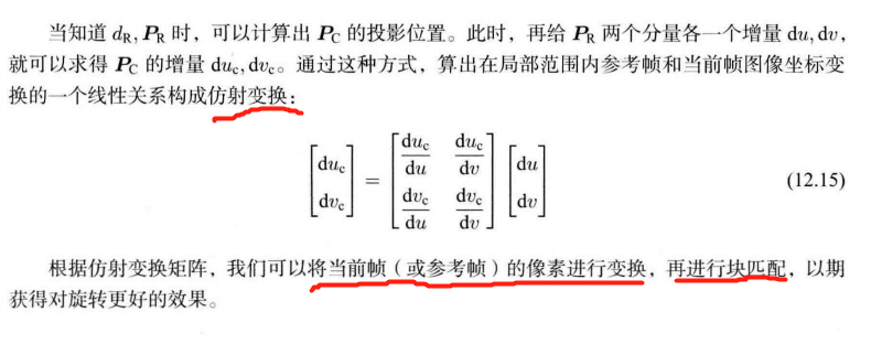
3、单目稠密重建从正深度 改成 逆深度,并添加仿射变换。
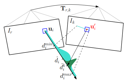
仿射变换用于 块匹配前,进一步考虑了相机发生运动的情形(当前帧和参考帧之间发行运动了),以期可以取得更好的 匹配效果。
实际的深度分布: 尾部稍长,负数区域为0 逆深度

ORB_SLAM2
题4
4、论证如何在八叉树中进行导航和路径规划
navigation based on octomap
导航:如何从地图中A点到B点。
- 如何在地图中地位自己(localization)
- 如何从 A 到 B 规划一条路径(planning), path planning 有global和local之分,同时都需要。global path planning有dijkstra,A* ,D*等算法。local path planning 有自适应动态窗法等。
Autonomous Navigation in Unknown Environments with Sparse Bayesian Kernel-based Occupancy Mapping
OctoMap:An Efficient Probabilistic 3D Mapping Framework Based on Octrees
找到了别的树
FAST-LIO2: Fast Direct LiDAR-inertial Odometry
题5
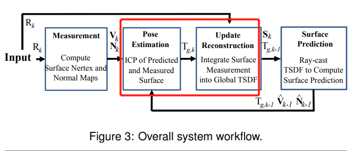
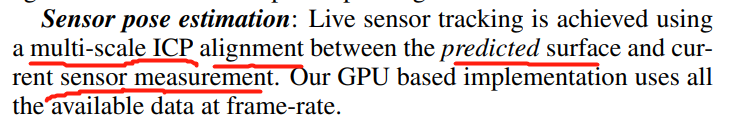
5、TSDF是如何进行位姿估计和更新的。
论文链接: KinectFusion: Real-Time Dense Surface Mapping and Tracking
题6
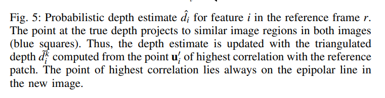
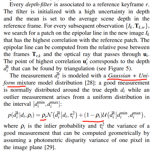
6、均匀-高斯混合滤波器的原理与实现
待做:
- 用数据集 跑源码
在12.2.3 节讨论了。P311
SVO源码链接
PDF链接:https://rpg.ifi.uzh.ch/docs/ICRA14_Forster.pdf
SVO 全称 Semi-direct monocular Visual Odometry(半直接视觉里程计)
点云 深度 概率模型是 高斯+均匀分布
瑞士苏黎世大学 机器人与感知小组http://rpg.ifi.uzh.ch。
https://github.com/uzh-rpg/rpg_svo/blob/master/svo/src/depth_filter.cpp
其它:
SVO的深度滤波器使用的概率模型是《Video-based, Real-Time Multi View Stereo》中的深度概率模型,不同的是SVO中的使用的逆深度估计。
Video-based, Real-Time Multi View Stereo》pdf链接