需要源码和数据集请点赞关注收藏后评论区留言或者私信~~~

一、威胁模型

对抗性机器学习，意思是在训练的模型中添加细微的扰动最后会导致模型性能的巨大差异，接下来我们通过一个图像分类器上的示例来进行讲解，具体的说，会使用第一个也是最流行的攻击方法之一，快速梯度符号攻击来欺骗一个MNIST分类器

每一类攻击都有不同的目标和对攻击者知识的假设，总的目标是在输入数据中添加最少的扰动，以导致所需要的错误分类。攻击有两者假设，分别是黑盒与白盒

1：白盒攻击假设攻击者具有对模型的全部知识和访问权，包括体系结构，输入，输出和权重。

2：黑盒攻击假设攻击者只访问模型的输入和输出，对底层架构或权重一无所知

FGSM攻击是一种以错误分类为目标的白盒攻击

二、快速梯度符号攻击简介 

FGSM直接利用神经网络的学习方式--梯度更新来攻击神经网络，这种攻击时根据相同的反向传播梯度调整输入数据来最大化损失，换句话说，攻击使用了输入数据相关的梯度损失方式，通过调整输入数据，使损失最大化。

三、输入

对抗样本模型只有三个输入 定义如下

1：epsilons 用于运行的epsilon值列表，在列表中保留0很重要，因为它代表原始测试集上的模型性能

2：pretrained_model  使用mnist训练的预训练MNIST模型的路径 可自行下载

3：use_cuda  布尔标志 如果需要和可用，则使用CUDA 其实不用也行 因为用CPU也不会花费太多时间

四、FGSM攻击 

介绍完上面的基本知识之后，可以通过干扰原始输入来定义创建对抗示例的函数，它需要三个输入分别为图像是干净的原始图像，epsilon是像素方向的扰动量，data_grad是输入图片

攻击函数代码如下

accuracies = []
examples = []

# Run test for each epsilon
for eps in epsilons:
    acc, ex = test(model, device, test_loader, eps)
    accuracies.append(acc)
    examples.append(ex)

运行攻击后输出如下

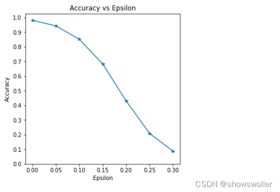
这里为epsilon输入中的每个值运行测试，随着值的增加，打印的精度逐渐降低

 五、结果分析

第一个结果是accuracy与参数曲线的关系，可以看到，随着参数的增加，我们期望测试精度会降低，这是因为较大的参数意味着我们朝着将损失最大化的方向迈出了更大的一步 结果如下

 六、对抗示例

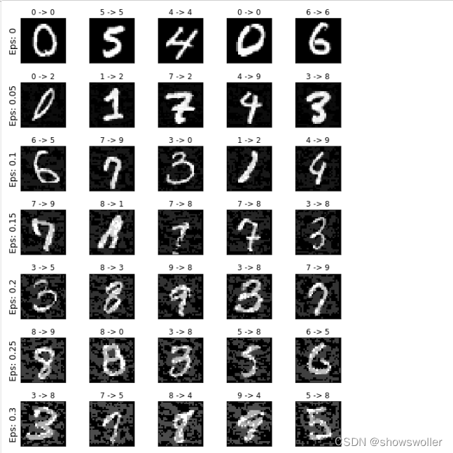
系统性学习过计算机的小伙伴们应该对tradeoff这个词并并不陌生，它意味着权衡，如上图所示，随着参数的增加，测试精度降低，但是同时扰动变得更加易于察觉，这里攻击者就要考虑准确性降低和可感知性之间的权衡。接下来将展示不同epsilon值的成功对抗

参数等于0时为原始干净且无扰动时的图像，可以看到，扰动在参数为0.15和0.3时变得明显

 七、代码

部分源码如下

# In[1]:


from __future__ import print_function
import torch
import torch.nn as nn
import torch.nn.functional as F
import torch.optim as optim
from torchvision import datasets, transforms
import numpy as np
import matplotlib.pyplot as plt





# 
# -  **pretrained_model** - path to the pretrained MNIST model which was
#    trained with
#    `pytorch/examples/mnist <https://github.com/pytorch/examples/tree/master/mnist>`__.
#    For simplicity, download the pretrained model `here <https://drive.google.com/drive/folders/1fn83DF14tWmit0RTKWRhPq5uVXt73e0h?usp=sharing>`__.
# 



# In[9]:


epsilons = [0, .05, .1, .15, .2, .25, .3]
pretrained_model = "data/lenet_mnist_model.pth"
use_cuda=True


# Model Under Attack
# ~~~~~~~~~~~~~~~~~~
# 
# As mentioned, the model under attack is the same MNIST model from
# `pytorch/examples/mnist <https://github.com/pytorch/examples/tree/master/mnist>`__.
# You may train and save your own MNIST model or you can download and use
# the provided model. The *Net* definition and test dataloader here have
# been copied from the MNIST example. The purpose of this section is to
# define the model and dataloader, then initialize the model and load the
# pretrained weights.
# 
# 
# 

# In[3]:


# LeNet Model definition

        super(Net, self).__init__()
        self.conv1 = nn.Conv2d(1, 10, kernel_size=5)
        self.conv2 = nn.Conv2d(10, 20, kernel_size=5)
        self.conv2_drop = nn.Dropout2d()
        self.fc1 = nn.Linear(320, 50)
        self.fc2 = nn.Linear(50, 10)

    d
        return F.log_softmax(x, dim=1)

# MNIST Test dataset and dataloader declaration
test_loader = torch.utils.data.DataLoader(
    datasets.MNIST('../data', train=False, download=True, transform=transforms.Compose([
            transforms.ToTensor(),
            ])), 
        batch_size=1, shuffle=True)

# Define what device we are using
print("CUDA Available: ",torch.cuda.is_available())
device = torch.device("cuda" if (use_cuda and torch.cuda.is_available()) else "cpu")

# Initialize the network
model = Net().to(device)

# Load the pretrained model
model.load_state_dict(torch.load(pretrained_model, map_location='cpu'))

# Set the model in evaluation mode. In this case this is for the Dropout layers
model.eval()


ginal inputs. The ``fgsm_attack`` function takes three
# inputs, *image* is the original clean image ($x$), *epsilon* is
# the pixel-wise perturbation amount ($\epsilon$), and *data_grad*
# is gradient of the loss w.r.t the input image
# ($\nabla_{x} J(\mathbf{\theta}, \mathbf{x}, y)$). The function
# then creates perturbed image as
# 
# \begin{align}perturbed\_image = image + epsilon*sign(data\_grad) = x + \epsilon * sign(\nabla_{x} J(\mathbf{\theta}, \mathbf{x}, y))\end{align}
# 
# Finally, in order to maintain the original range of the data, the
# perturbed image is clipped to range $[0,1]$.
# 
# 
# 

# In[4]:


#= data_grad.sign()
    # Create the perturbed image by adjusting each pixel of the input image
    perturbed_image = image + epsilon*sign_data_grad
    # Adding clipping to maintain [0,1] range
    perturbed_image = torch.clamp(perturbed_image, 0, 1)
    # Return the perturbed image
    return perturbed_image


# Testing Function
# ~~~~~~~~~~~~~~~~
# 
# Finally, the central result of this tutorial comes from the ``test``
# function. Each call to this test function performs a full test step on
# the MNIST test set and reports a final accuracy. However, notice that
# this function also takes an *epsilon* input. This is because the
# ``test`` function reports the accuracy of a model that is under attack
# from an adversary with strength $\epsilon$. More specifically, for
# each sample in the test set, the function computes the gradient of the
# loss w.r.t the input data ($data\_grad$), creates a perturbed
# image with ``fgsm_attack`` ($perturbed\_data$), then checks to see
# if the perturbed example is adversarial. In addition to testing the
# accuracy of the model, the function also saves and returns some
# successful adversarial examples to be visualized later.
# 
# 
# 

# In[5]:


t = data.to(device), target.to(device)

        # Set requires_grad attribute of tensor. Important for Attack
        data.requires_grad = True

        # Forward pass the data through the model
        output = model(data)
        init_pred = output.max(1, keepdim=True)[1] # get the index of the max log-probability

        # If the initial prediction is wrong, dont bother attacking, just move on
        if init_pred.item() != target.item():
            continue

        # Calculate the loss
        loss = F.nll_loss(output, target)

        # Zero all existing gradients
        model.zero_grad()

        # Calculate gradients of model in backward pass
        loss.backward()

        # Collect datagrad
        data_grad = data.grad.data

        # Call FGSM Attack
        perturbed_data = fgsm_attack(data, epsilon, data_grad)

        # Re-classify the perturbed image
        output = model(perturbed_data)

        # Check for success
        final_pred = output.max(1, keepdim=True)[1] # get the index of the max log-probability
        if final_pred.item() == target.item():
            correct += 1
            # Special case for saving 0 epsilon examples
            if (epsilon == 0) and (len(adv_examples) < 5):
                adv_ex = perturbed_data.squeeze().detach().cpu().numpy()
                adv_examples.append( (init_pred.item(), final_pred.item(), adv_ex) )
        else:
            # Save some adv examples for visualization later
            if len(adv_examples) < 5:
                adv_ex = perturbed_data.squeeze().detach().cpu().numpy()
                adv_examples.append( (init_pred.item(), final_pred.item(), adv_ex) )

    # Calculate final accuracy for this epsilon
    final_acc = correct/float(len(test_loader))
    print("Epsilon: {}\tTest Accuracy = {} / {} = {}".format(epsilon, correct, len(test_loader), final_acc))
al_acc, adv_examples


# Run Attack
# ~~~~~~~~~~
# 
# The last part of the implementation is to actually run the attack. Here,
# we run a full test step for each epsilon value in the *epsilons* input.
# For each epsilon we also save the final accuracy and some successful
# adversarial examples to be plotted in the coming sections. Notice how
# the printed accuracies decrease as the epsilon value increases. Also,
# note the $\epsilon=0$ case represents the original test accuracy,
# with no attack.
# 
# 
# 

# In[6]:


accuracies = []
examples = []

# Run test for each epsilon
for eps in epsilons:
    acc, ex = test(model, device, test_loader, eps)
    accuracies.append(acc)
    examples.append(ex)


# Results
# -------
# 
# Accuracy vs Epsilon
# ~~~~~~~~~~~~~~~~~~~
# 
# The first result is the accuracy versus epsilon plot. As alluded to
# earlier, as epsilon increases we expect the test accuracy to decrease.
# This is because larger epsilons mean we take a larger step in the
# direction that will maximize the loss. Notice the trend in the curve is
# not linear even though the epsilon values are linearly spaced. For
# example, the accuracy at $\epsilon=0.05$ is only about 4% lower
# than $\epsilon=0$, but the accuracy at $\epsilon=0.2$ is 25%
# lower than $\epsilon=0.15$. Also, notice the accuracy of the model
# hits random accuracy for a 10-class classifier between
# $\epsilon=0.25$ and $\epsilon=0.3$.
# 
# 
# 

# In[10]:


plt.figure(figsize=(5,5))
plt.plot(epsilons, accuracies, "*-")
plt.yticks(np.arange(0, 1.1, step=0.1))
plt.xticks(np.arange(0, .35, step=0.05))
plt.title("Accuracy vs Epsilon")
plt.xlabel("Epsilon")
plt.ylabel("Accuracy")
plt.show()


# Sample Adversarial Examples
# ~~~~~~~~~~~~~~~~~~~~~~~~~~~
# 
# Remember the idea of no free lunch? In this case, as epsilon increases
# the test accuracy decreases **BUT** the perturbations become more easily
# perceptible. In reality, there is a tradeoff between accuracy
# degredation and perceptibility that an attacker must consider. Here, we
# show some examples of successful adversarial examples at each epsilon
# value. Each row of the plot shows a different epsilon value. The first
# row is the $\epsilon=0$ examples which represent the original
# “clean” images with no perturbation. The title of each image shows the
# “original classification -> adversarial classification.” Notice, the
# perturbations start to become evident at $\epsilon=0.15$ and are
# quite evident at $\epsilon=0.3$. However, in all cases humans are
# still capable of identifying the correct class despite the added noise.
# 
# 
# 

# In[11]:


# Plot several examples of adversarial samples at each epsilon
cnt = 0
plt.figure(figsize=(8,10))
for i in range(len(epsilons)):
    for j in range(len(examples[i])):
        cnt += 1
        plt.subplot(len(epsilons),len(examples[0]),cnt)
        plt.xticks([], [])
        plt.yticks([], [])
        if j == 0:
            plt.ylabel("Eps: {}".format(epsilons[i]), fontsize=14)
        orig,adv,ex = examples[i][j]
        plt.title("{} -> {}".format(orig, adv))
        plt.imshow(ex, cmap="gray")
plt.tight_layout()
plt.show()


# Where to go next?
# -----------------
# 
# Hopefully this tutorial gives some insight into the topic of adversarial
# machine learning. There are many potential directions to go from here.
# This attack represents the very beginning of adversarial attack research
# and since there have been many subsequent ideas for how to attack and
# defend ML models from an adversary. In fact, at NIPS 2017 there was an
# adversarial attack and defense competition and many of the methods used
# in the competition are described in this paper: `Adversarial Attacks and
# Defences Competition <https://arxiv.org/pdf/1804.00097.pdf>`__. The work
# on defense also leads into the idea of making machine learning models
# more *robust* in general, to both naturally perturbed and adversarially
# crafted inputs.
# 
# Another direction to go is adversarial attacks and defense in different
# domains. Adversarial research is not limited to the image domain, check
# out `this <https://arxiv.org/pdf/1801.01944.pdf>`__ attack on
# speech-to-text models. But perhaps the best way to learn more about
# adversarial machine learning is to get your hands dirty. Try to
# implement a different attack from the NIPS 2017 competition, and see how
# it differs from FGSM. Then, try to defend the model from your own
# attacks.
# 
# 
# 

创作不易 觉得有帮助请点赞关注收藏~~~