文章目录
- 0 前言
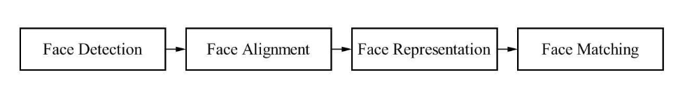
- 1 机器学习-人脸识别过程
- 人脸检测
- 人脸对其
- 人脸特征向量化
- 人脸识别
- 2 深度学习-人脸识别过程
- 人脸检测
- 人脸识别
- Metric Larning
- 3 最后
0 前言
🔥 优质竞赛项目系列,今天要分享的是
🚩 深度学习 机器视觉 人脸识别系统
该项目较为新颖,适合作为竞赛课题方向,学长非常推荐!
🥇学长这里给一个题目综合评分(每项满分5分)
- 难度系数:3分
- 工作量:3分
- 创新点:3分
🧿 更多资料, 项目分享:
https://gitee.com/dancheng-senior/postgraduate
1 机器学习-人脸识别过程
基于传统图像处理和机器学习技术的人脸识别技术,其中的流程都是一样的。
机器学习-人脸识别系统都包括:
- 人脸检测
- 人脸对其
- 人脸特征向量化
- 人脸识别
人脸检测
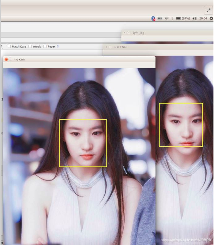
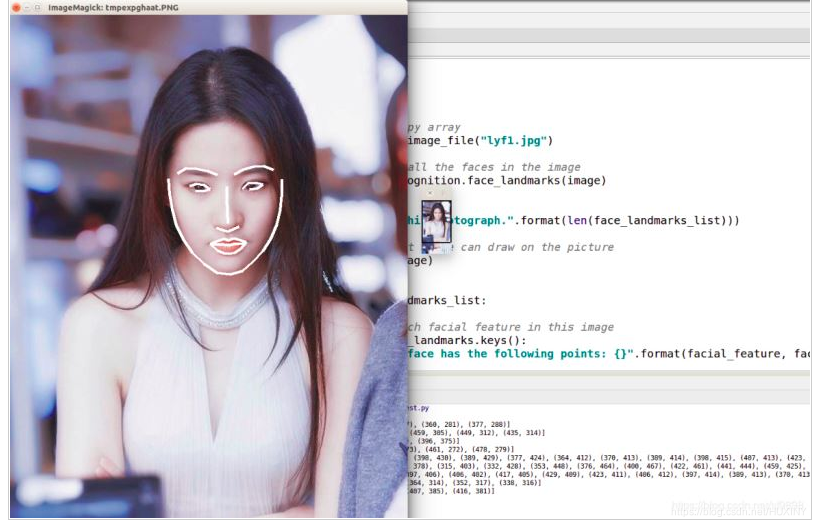
人脸检测用于确定人脸在图像中的大小和位置,即解决“人脸在哪里”的问题,把真正的人脸区域从图像中裁剪出来,便于后续的人脸特征分析和识别。下图是对一张图像的人脸检测结果:
人脸对其
同一个人在不同的图像序列中可能呈现出不同的姿态和表情,这种情况是不利于人脸识别的。
所以有必要将人脸图像都变换到一个统一的角度和姿态,这就是人脸对齐。
它的原理是找到人脸的若干个关键点(基准点,如眼角,鼻尖,嘴角等),然后利用这些对应的关键点通过相似变换(Similarity
Transform,旋转、缩放和平移)将人脸尽可能变换到标准人脸。
下图是一个典型的人脸图像对齐过程:
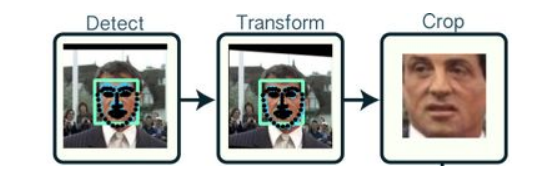
这幅图就更加直观了:

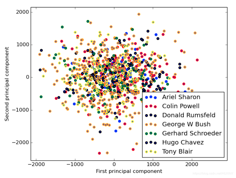
人脸特征向量化
这一步是将对齐后的人脸图像,组成一个特征向量,该特征向量用于描述这张人脸。
但由于,一幅人脸照片往往由比较多的像素构成,如果以每个像素作为1维特征,将得到一个维数非常高的特征向量, 计算将十分困难;而且这些像素之间通常具有相关性。
所以我们常常利用PCA技术对人脸描述向量进行降维处理,保留数据集中对方差贡献最大的人脸特征来达到简化数据集的目的
PCA人脸特征向量降维示例代码:
#coding:utf-8
from numpy import *
from numpy import linalg as la
import cv2
import os

def loadImageSet(add):
    FaceMat = mat(zeros((15,98*116)))
    j =0
    for i in os.listdir(add):
        if i.split('.')[1] == 'normal':
            try:
                img = cv2.imread(add+i,0)
            except:
                print 'load %s failed'%i
            FaceMat[j,:] = mat(img).flatten()
            j += 1
    return FaceMat

def ReconginitionVector(selecthr = 0.8):
    # step1: load the face image data ,get the matrix consists of all image
    FaceMat = loadImageSet('D:\python/face recongnition\YALE\YALE\unpadded/').T
    # step2: average the FaceMat
    avgImg = mean(FaceMat,1)
    # step3: calculate the difference of avgimg and all image data(FaceMat)
    diffTrain = FaceMat-avgImg
    #step4: calculate eigenvector of covariance matrix (because covariance matrix will cause memory error)
    eigvals,eigVects = linalg.eig(mat(diffTrain.T*diffTrain))
    eigSortIndex = argsort(-eigvals)
    for i in xrange(shape(FaceMat)[1]):
        if (eigvals[eigSortIndex[:i]]/eigvals.sum()).sum() >= selecthr:
            eigSortIndex = eigSortIndex[:i]
            break
    covVects = diffTrain * eigVects[:,eigSortIndex] # covVects is the eigenvector of covariance matrix
    # avgImg 是均值图像,covVects是协方差矩阵的特征向量,diffTrain是偏差矩阵
    return avgImg,covVects,diffTrain

def judgeFace(judgeImg,FaceVector,avgImg,diffTrain):
    diff = judgeImg.T - avgImg
    weiVec = FaceVector.T* diff
    res = 0
    resVal = inf
    for i in range(15):
        TrainVec = FaceVector.T*diffTrain[:,i]
        if  (array(weiVec-TrainVec)**2).sum() < resVal:
            res =  i
            resVal = (array(weiVec-TrainVec)**2).sum()
    return res+1

if __name__ == '__main__':

    avgImg,FaceVector,diffTrain = ReconginitionVector(selecthr = 0.9)
    nameList = ['01','02','03','04','05','06','07','08','09','10','11','12','13','14','15']
    characteristic = ['centerlight','glasses','happy','leftlight','noglasses','rightlight','sad','sleepy','surprised','wink']

    for c in characteristic:

        count = 0
        for i in range(len(nameList)):

            # 这里的loadname就是我们要识别的未知人脸图,我们通过15张未知人脸找出的对应训练人脸进行对比来求出正确率
            loadname = 'D:\python/face recongnition\YALE\YALE\unpadded\subject'+nameList[i]+'.'+c+'.pgm'
            judgeImg = cv2.imread(loadname,0)
            if judgeFace(mat(judgeImg).flatten(),FaceVector,avgImg,diffTrain) == int(nameList[i]):
                count += 1
        print 'accuracy of %s is %f'%(c, float(count)/len(nameList))  # 求出正确率
人脸识别
这一步的人脸识别,其实是对上一步人脸向量进行分类,使用各种分类算法。
比如:贝叶斯分类器,决策树,SVM等机器学习方法。
从而达到识别人脸的目的。
这里分享一个svm训练的人脸识别模型:
    from __future__ import print_function

    from time import time
    import logging
    import matplotlib.pyplot as plt

    from sklearn.cross_validation import train_test_split
    from sklearn.datasets import fetch_lfw_people
    from sklearn.grid_search import GridSearchCV
    from sklearn.metrics import classification_report
    from sklearn.metrics import confusion_matrix
    from sklearn.decomposition import RandomizedPCA
    from sklearn.svm import SVC


    print(__doc__)

    # Display progress logs on stdout
    logging.basicConfig(level=logging.INFO, format='%(asctime)s %(message)s')


    ###############################################################################
    # Download the data, if not already on disk and load it as numpy arrays

    lfw_people = fetch_lfw_people(min_faces_per_person=70, resize=0.4)

    # introspect the images arrays to find the shapes (for plotting)
    n_samples, h, w = lfw_people.images.shape

    # for machine learning we use the 2 data directly (as relative pixel
    # positions info is ignored by this model)
    X = lfw_people.data
    n_features = X.shape[1]

    # the label to predict is the id of the person
    y = lfw_people.target
    target_names = lfw_people.target_names
    n_classes = target_names.shape[0]

    print("Total dataset size:")
    print("n_samples: %d" % n_samples)
    print("n_features: %d" % n_features)
    print("n_classes: %d" % n_classes)


    ###############################################################################
    # Split into a training set and a test set using a stratified k fold

    # split into a training and testing set
    X_train, X_test, y_train, y_test = train_test_split(
        X, y, test_size=0.25, random_state=42)


    ###############################################################################
    # Compute a PCA (eigenfaces) on the face dataset (treated as unlabeled
    # dataset): unsupervised feature extraction / dimensionality reduction
    n_components = 80

    print("Extracting the top %d eigenfaces from %d faces"
          % (n_components, X_train.shape[0]))
    t0 = time()
    pca = RandomizedPCA(n_components=n_components, whiten=True).fit(X_train)
    print("done in %0.3fs" % (time() - t0))

    eigenfaces = pca.components_.reshape((n_components, h, w))

    print("Projecting the input data on the eigenfaces orthonormal basis")
    t0 = time()
    X_train_pca = pca.transform(X_train)
    X_test_pca = pca.transform(X_test)
    print("done in %0.3fs" % (time() - t0))

    ###############################################################################
    # Train a SVM classification model

    print("Fitting the classifier to the training set")
    t0 = time()
    param_grid = {'C': [1,10, 100, 500, 1e3, 5e3, 1e4, 5e4, 1e5],
                  'gamma': [0.0001, 0.0005, 0.001, 0.005, 0.01, 0.1], }
    clf = GridSearchCV(SVC(kernel='rbf', class_weight='balanced'), param_grid)
    clf = clf.fit(X_train_pca, y_train)
    print("done in %0.3fs" % (time() - t0))
    print("Best estimator found by grid search:")
    print(clf.best_estimator_)

    print(clf.best_estimator_.n_support_)
    ###############################################################################
    # Quantitative evaluation of the model quality on the test set

    print("Predicting people's names on the test set")
    t0 = time()
    y_pred = clf.predict(X_test_pca)
    print("done in %0.3fs" % (time() - t0))

    print(classification_report(y_test, y_pred, target_names=target_names))
    print(confusion_matrix(y_test, y_pred, labels=range(n_classes)))


    ###############################################################################
    # Qualitative evaluation of the predictions using matplotlib

    def plot_gallery(images, titles, h, w, n_row=3, n_col=4):
        """Helper function to plot a gallery of portraits"""
        plt.figure(figsize=(1.8 * n_col, 2.4 * n_row))
        plt.subplots_adjust(bottom=0, left=.01, right=.99, top=.90, hspace=.35)
        for i in range(n_row * n_col):
            plt.subplot(n_row, n_col, i + 1)
            # Show the feature face
            plt.imshow(images[i].reshape((h, w)), cmap=plt.cm.gray)
            plt.title(titles[i], size=12)
            plt.xticks(())
            plt.yticks(())

    # plot the result of the prediction on a portion of the test set

    def title(y_pred, y_test, target_names, i):
        pred_name = target_names[y_pred[i]].rsplit(' ', 1)[-1]
        true_name = target_names[y_test[i]].rsplit(' ', 1)[-1]
        return 'predicted: %s\ntrue:      %s' % (pred_name, true_name)

    prediction_titles = [title(y_pred, y_test, target_names, i)
                         for i in range(y_pred.shape[0])]

    plot_gallery(X_test, prediction_titles, h, w)

    # plot the gallery of the most significative eigenfaces

    eigenface_titles = ["eigenface %d" % i for i in range(eigenfaces.shape[0])]
    plot_gallery(eigenfaces, eigenface_titles, h, w)

    plt.show()
2 深度学习-人脸识别过程
不同于机器学习模型的人脸识别,深度学习将人脸特征向量化,以及人脸向量分类结合到了一起,通过神经网络算法一步到位。
深度学习-人脸识别系统都包括:
- 人脸检测
- 人脸对其
- 人脸识别
人脸检测
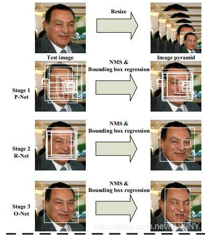
深度学习在图像分类中的巨大成功后很快被用于人脸检测的问题,起初解决该问题的思路大多是基于CNN网络的尺度不变性,对图片进行不同尺度的缩放,然后进行推理并直接对类别和位置信息进行预测。另外,由于对feature
map中的每一个点直接进行位置回归,得到的人脸框精度比较低,因此有人提出了基于多阶段分类器由粗到细的检测策略检测人脸,例如主要方法有Cascade CNN、
DenseBox和MTCNN等等。
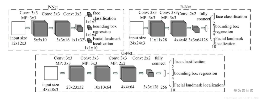
MTCNN是一个多任务的方法,第一次将人脸区域检测和人脸关键点检测放在了一起,与Cascade
CNN一样也是基于cascade的框架,但是整体思路更加的巧妙合理,MTCNN总体来说分为三个部分:PNet、RNet和ONet,网络结构如下图所示。
人脸识别
人脸识别问题本质是一个分类问题,即每一个人作为一类进行分类检测,但实际应用过程中会出现很多问题。第一,人脸类别很多,如果要识别一个城镇的所有人,那么分类类别就将近十万以上的类别,另外每一个人之间可获得的标注样本很少,会出现很多长尾数据。根据上述问题,要对传统的CNN分类网络进行修改。
我们知道深度卷积网络虽然作为一种黑盒模型,但是能够通过数据训练的方式去表征图片或者物体的特征。因此人脸识别算法可以通过卷积网络提取出大量的人脸特征向量,然后根据相似度判断与底库比较完成人脸的识别过程,因此算法网络能不能对不同的人脸生成不同的特征,对同一人脸生成相似的特征,将是这类embedding任务的重点,也就是怎么样能够最大化类间距离以及最小化类内距离。
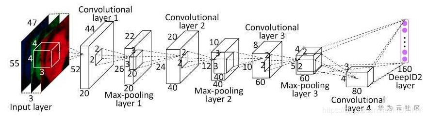
Metric Larning
深度学习中最先应用metric
learning思想之一的便是DeepID2了。其中DeepID2最主要的改进是同一个网络同时训练verification和classification(有两个监督信号)。其中在verification
loss的特征层中引入了contrastive loss。
Contrastive
loss不仅考虑了相同类别的距离最小化,也同时考虑了不同类别的距离最大化,通过充分运用训练样本的label信息提升人脸识别的准确性。因此,该loss函数本质上使得同一个人的照片在特征空间距离足够近,不同人在特征空间里相距足够远直到超过某个阈值。(听起来和triplet
loss有点像)。
3 最后
🧿 更多资料, 项目分享:
https://gitee.com/dancheng-senior/postgraduate


![[ROS2系列] ubuntu 20.04测试rtabmap 3D建图(二)](https://img-blog.csdnimg.cn/f01360f12f9b4ad7854fea51c0e87f76.png)