在本文中，我们将使用 CNN （卷积神经网络）和机器学习分类器创建一个检测一个人是否戴着口罩的分类器。它将检测一个人是否戴着口罩。

我们将从头开始学习，我将对每一步进行解释。我需要你对机器学习和数据科学有基本的了解。我已经在本地 Windows 10 机器上实现了它，如果你愿意，你也可以在 Google Colab 上实现它。

卷积神经网络是一种人工神经网络，旨在处理像素数据。它们经常用于图像处理和图像识别。

图 1 戴口罩 V/S 没戴口罩

CNN 模型管道

首先，我们将输入大小为 224×224 像素的 RGB 图像。然后这些图像将进入一个 CNN 模型，从中提取 128 个相关的特征向量。然后我们将使用这些特征向量来训练我们的各种机器学习分类器，如逻辑回归、随机森林等，以分类该图像中的人是否戴着口罩。你可以参考下图以获得更好的理解。

图 2 解释我们的整个机器学习管道

让我们开始吧

技术提升

本文由技术群粉丝投稿分享，项目源码、数据、技术交流提升，均可加交流群获取，群友已超过2000人，添加时最好的备注方式为：来源+兴趣方向，方便找到志同道合的朋友

方式①、添加微信号：dkl88191，备注：来自CSDN +研究方向
方式②、微信搜索公众号：Python学习与数据挖掘，后台回复：加群

训练 CNN 模型的代码工作

在本节中，我们将学习编码部分。

我们将讨论数据集的加载和预处理、训练 CNN 模型以及提取特征向量以训练机器学习分类器。

导入必要的库：

我们将导入此项目所需的所有必要库。

我们将使用 Numpy ，用于执行复杂的数学计算。Pandas 加载和预处理数据集。

import numpy as np  
import pandas as pd  
import matplotlib.pyplot as plt  
import os  
  
from itertools import cycle  
from sklearn.model_selection import train_test_split  
from tensorflow.keras.models import Model  
from tensorflow.keras.layers import Dropout, Dense, AveragePooling2D, Flatten ,Dense, Input  
from sklearn.metrics import classification_report, confusion_matrix  
  
import cv2  

from sklearn.metrics import roc_curve, auc  
from sklearn.preprocessing import label_binarize  
  
from scipy import interp  
from sklearn.ensemble import RandomForestClassifier  
  
from tensorflow.keras.preprocessing.image import ImageDataGenerator  
from tensorflow.keras.applications import MobileNetV2  
from tensorflow.keras.optimizers import Adam  

数据集的加载和预处理

你可以从该 GitHub Repo 下载数据集：https://github.com/prajnasb/observations/tree/master/experiements

从上述存储库中克隆数据集。

该数据集包含 1200 多张不同人是否戴口罩的图像。加载数据集后，我们将对其进行预处理。

预处理涉及拆分训练和测试数据集，将像素值转换为 0 到 1 之间，并将标签转换为 one-hot 编码标签。

下面是加载和预处理数据集的代码。它的注释很完整，你可以轻松理解它。

显示训练和测试集

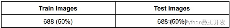
在下面的代码中，我们将首先从文件夹中读取所有图像，然后通过将它们调整为 224×224 像素将它们存储在一个数组中。之后，我们将标记这些图像。带有口罩的图像有一个标签 0，没有口罩的图像有一个标签 1。最后，我们将使用名为 train test split 的 sklearn 函数将此数据集拆分为训练和测试。

# 列出主目录中所有带口罩的图像。

filenames = os.listdir("observations-master/experiements/data/with_mask")  
np.random.shuffle(filenames)  
print(filenames) # Read all the images from that directory and resize them into 224x224 pixels.  
  
with_mask_data = [cv2.resize(cv2.imread("observations-master/experiements/data/with_mask/"+img), (224,224)) for img in filenames]  
print(len(with_mask_data))  

# 对于不包含口罩的图像，执行上述类似步骤。

filenames = os.listdir("observations-master/experiements/data/without_mask")  
np.random.shuffle(filenames)  
print(filenames)  
  
without_mask_data = [cv2.resize(cv2.imread("observations-master/experiements/data/without_mask/"+img), (224,224)) for img in filenames]  
print(len(without_mask_data))  

# 我们将两个数组组合成一个数组，通过将它们除以 255 将每个像素值在 0 和 1 之间转换。

data = np.array(with_mask_data + without_mask_data).astype('float32')/255 # Label of the image with a mask - 0 # Label of the image without mask - 1  
labels = np.array([0]*len(with_mask_data) + [1]*len(without_mask_data))  
print(data.shape) # Splitting the data into training and testing sets.  
  
(training_data, testing_data, training_label, testing_label) = train_test_split(data, labels, test_size=0.50, stratify=labels, random_state=42)  

print(training_data.shape) # Function to Plot the Accuracy/Loss Curves  
  
def plot_acc_loss(result, epochs):  
acc = result.history['accuracy']  
loss = result.history['loss']  
  
val_acc = result.history['val_accuracy']  
val_loss = result.history['val_loss']  
  
plt.figure(figsize=(15, 5))  
plt.subplot(121)  
plt.plot(range(1,epochs), acc[1:], label='Train_acc')  
plt.plot(range(1,epochs), val_acc[1:], label='Val_acc')  
  
plt.title('Accuracy over ' + str(epochs) + ' Epochs', size=15)  
plt.legend()  
  
plt.grid(True)  
plt.subplot(122)  
plt.plot(range(1,epochs), loss[1:], label='Train_loss')  
plt.plot(range(1,epochs), val_loss[1:], label='Val_loss')  
  
plt.title('Loss over ' + str(epochs) + ' Epochs', size=15)  
plt.legend()  
plt.grid(True)  
plt.show()  

构建卷积神经网络 (CNN)

现在我们将构建我们的卷积神经网络。首先，我们使用图像数据生成器来增加数据集中的图像数量。该图像生成器将从这些现有图像中生成更多照片。它执行顺时针或逆时针旋转，改变对比度，执行放大或缩小等。

之后，我们将使用预训练的 MobileNetV2 架构来训练我们的模型。它是一种迁移学习模型。迁移学习是使用预训练模型来训练新的深度学习模型，即如果两个模型执行相似的任务，我们可以共享知识。

应用迁移学习后，我们将应用展平层将 2D 矩阵转换为 1D 数组。之后，我们将应用 dense 层和 dropout 层来执行分类。

最后，我们将批量大小设为 32，epoch 数设为 25 来训练我们的模型。你可以根据自己的计算能力取其他值。

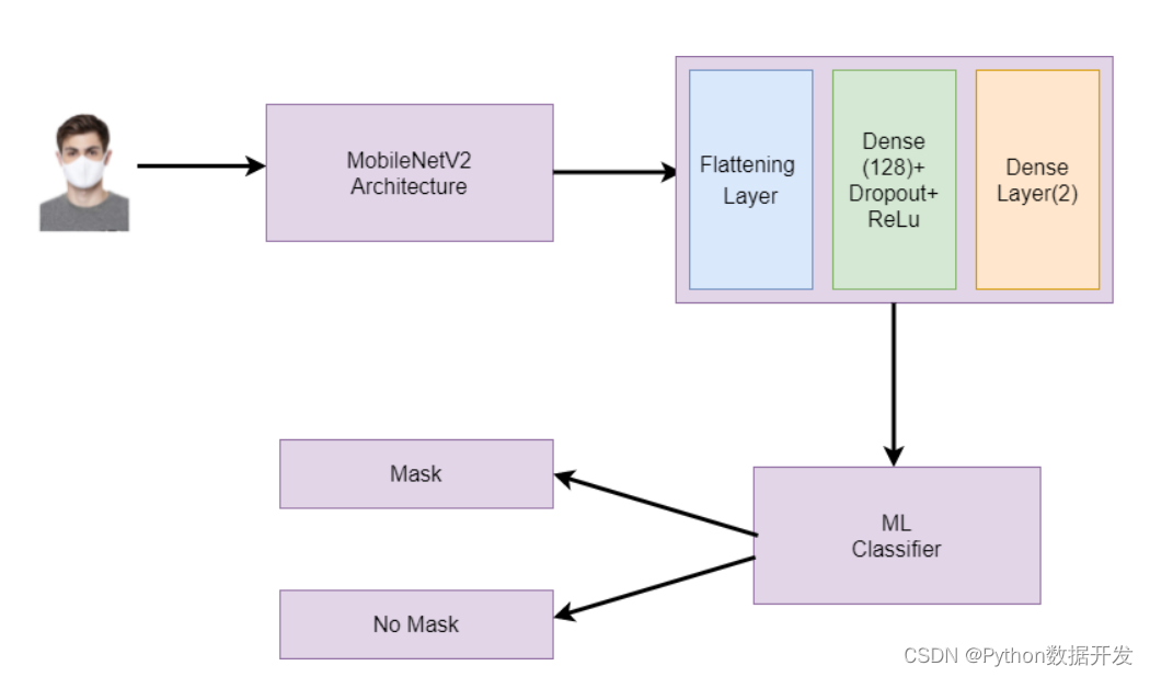
图 3 解释我们的卷积神经网络

训练卷积神经网络模型的代码：

我们将构建我们的迁移学习 MobileNetV2 架构，这是一个预训练的 CNN 模型。

首先，我们将使用图像数据生成器 ImageDataGenerator 从我们的数据集中生成更多图像。

之后，我们将设置我们的超参数，例如学习率、批量大小、epoch 数量等。

最后，我们将训练我们的模型并在测试集上检查它的准确性。

# Image data generator to generate more images.   
generator = ImageDataGenerator(  
rotation_range=20,  
zoom_range=0.15,  
width_shift_range=0.2,  
height_shift_range=0.2,  
shear_range=0.15,  
horizontal_flip=True,  
fill_mode="nearest")  

# Setting the hyperparameters.  
learning_rate = 0.0001  
epoch = 25  
batch_size = 32  

# Training the mobile net v2 architecture.  
transfer_learning_model = MobileNetV2(weights="imagenet", include_top=False,  
input_tensor=Input(shape=(224, 224, 3)))  
  
model_main = transfer_learning_model.output  
model_main = AveragePooling2D(pool_size=(7, 7))(model_main) # Applying the flattening layer.  
model_main = Flatten(name="flatten")(model_main)  
model_main = Dense(128, activation="relu", name="dense_layer")(model_main)  
model_main = Dropout(0.5)(model_main)  
model_main = Dense(2, activation="softmax")(model_main)  
cnn = Model(inputs=transfer_learning_model.input, outputs=model_main)  
  
for row in transfer_learning_model.layers:  
row.trainable = False  
optimizer = Adam(lr=learning_rate, decay=learning_rate / epoch)  
cnn.compile(loss="sparse_categorical_crossentropy", optimizer=optimizer,  
metrics=["accuracy"])  

# Train the CNN model  
history = cnn.fit(  
generator.flow(training_data, training_label, batch_size=batch_size),  
steps_per_epoch=len(training_data) // batch_size,  
validation_data=(testing_data, testing_label),  
validation_steps=len(testing_data) // batch_size,  
epochs=epoch)  

# Evaluate the trained model  
# Evaluate the model on the test set.  
  
cnn.evaluate(testing_data, testing_label)  
  
plot_acc_loss(history, 25)  

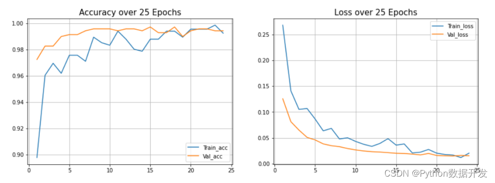
图 4 超过 25 个 epoch 的准确率和损失

我们在测试集上获得了 99.42% 的准确率

使用机器学习分类器

现在，我们将从之前训练的 CNN 模型中提取 128 个相关特征向量，并将它们应用于不同的 ML 分类器。我们将使用以下机器学习分类器：

EXtreme Gradient Boosting：

Extreme Gradient Boosting (XGBoost) 是一个开源库，可以高效地实现梯度提升算法。

首先，导入必要的库，然后将分类器定义为 XGBClassifier。拟合后，表示预测和准确度得分。我们得到准确率、混淆矩阵和分类报告作为输出。在这里，我们得到了 98.98% 的准确率。

随机森林分类器：

随机森林是一个分类器，它在给定数据集的不同子集上包含多个决策树，并取平均值以提高该数据集的预测准确性。森林中的树木数量越多，精度越高，并且可以防止过度拟合的问题。

首先，导入必要的库，然后将分类器定义为 RandomForestClassifier。拟合后，我们得到准确率、混淆矩阵和分类报告作为输出。在这里，我们的准确率达到了 99.41%，超过了 XGBoost。

逻辑回归：

逻辑回归是一种监督学习分类算法，用于预测目标变量的概率。目标或因变量的性质是二分类的，这意味着只有两个可能的类别。在这里，我们的准确率达到了 99.70%，高于 XGBoost，但略低于随机森林。

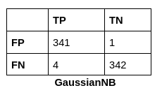
高斯分布：

正态分布也称为高斯分布。它表明接近平均值的数据比远离平均值的数据更频繁地出现。钟形曲线表示图形上的正态分布。

下面是提取基本特征向量并将这些特征向量放入机器学习分类器的代码。

在训练我们的 CNN 模型之后，我们现在将应用特征提取，并从这些图像中提取 128 个相关的特征向量。这些适当的特征向量被输入到我们的各种机器学习分类器中，以执行最终分类。

我们使用了各种机器学习模型，例如 XGBoost、随机森林、逻辑回归、GaussianNB 等。我们将选择能够提供最佳准确度的模型。

from keras.models import Model  
  
layer_name='dense_layer' # Extracting the layer from the above CNN model, which contains 128neurons.  
new_model = Model(inputs=cnn.input,  
  
outputs=cnn.get_layer(layer_name).output)  
new_model.summary()  

# Get new training data that only contains these 128 features.  
training_image_features = new_model.predict(training_data)  
training_image_features = pd.DataFrame(data=training_image_features)  
  
testing_image_features = new_model.predict(testing_data)  
testing_image_features = pd.DataFrame(data=testing_image_features)  

# Perform the classification using XGBoost Classifier. from xgboost import XGBClassifier  
  
from sklearn.metrics import accuracy_score  
  
classifier = XGBClassifier()  
classifier.fit(training_image_features, training_label)  
  
predictions = classifier.predict(testing_image_features) # Getting the accuracy score  
accuracy = accuracy_score(predictions, testing_label)  
print(f'{accuracy*100}%') # Getting the confusion matrix.  
  
cf = confusion_matrix(predictions, testing_label)  
print(cf)  
  
from sklearn.metrics import classification_report  
  
c_r = classification_report(predictions, testing_label, output_dict=True)  
print(c_r)  

# Perform the classification using RandomForest Classifier.  
  
from sklearn.ensemble import RandomForestClassifier  
  
rfc = RandomForestClassifier()  
rfc.fit(training_image_features, training_label)  
  
prediction = rfc.predict(testing_image_features)  
accuracy = accuracy_score(prediction, testing_label)  
print(f'{accuracy*100}%')  
  
cf = confusion_matrix(prediction, testing_label)  
print(cf)  
  
from sklearn.metrics import classification_report  
c_r = classification_report(prediction, testing_label, output_dict=True)  
  
print(c_r)  

# Perform the classification using LogisticRegression  
  
from sklearn.linear_model import LogisticRegression  
  
lin_r = LogisticRegression()  
lin_r.fit(training_image_features, training_label)  
  
prediction = lin_r.predict(testing_image_features)  
accuracy = accuracy_score(prediction, testing_label)  
print(f'{accuracy*100}%')  
  
cf = confusion_matrix(prediction, testing_label)  
print(cf)  
  
from sklearn.metrics import classification_report  
  
c_r = classification_report(prediction, testing_label, output_dict=True)  
print(c_r)  

# Perform the classification using GaussianNB  
  
from sklearn.naive_bayes import GaussianNB  
  
n_b = GaussianNB()  
n_b.fit(training_image_features, training_label)  
  
prediction = n_b.predict(testing_image_features)  
accuracy = accuracy_score(prediction, testing_label)  
print(f'{accuracy*100}%')  
  
cf = confusion_matrix(prediction, testing_label)  
print(cf)  
  
from sklearn.metrics import classification_report  
c_r = classification_report(prediction, testing_label, output_dict=True)  
print(c_r)  

结果

在本节中，我们将讨论我们的分类结果。我们将讨论我们达到了多少准确度，以及召回率和 f1 分数是多少。

Accuracy： 评估分类模型的一个参数是 Accuracy（准确度）。我们的模型正确预测的预测百分比称为准确度。以下是准确度的官方定义：准确预测的数量除以样本总数。

Precision： 被分类器判定的阳性样本中真阳性样本的比重

**F1 分数：**机器学习中最重要的评估指标之一是 F1 分数。结合了准确率和召回率，它是一个很好的综合指标。

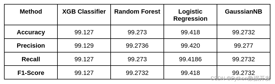
以下是我们用来训练模型的所有机器学习分类器的性能得分。逻辑回归给出的准确率最高，为 99.709%。

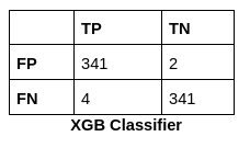
所有机器学习分类器的混淆矩阵是：混淆矩阵是一个总结预测结果的 NxN 矩阵。它包含每个类别的正确和错误预测的数量。

.png)

完整代码

在本节中，我分享了该项目中使用的完整代码。除了上述代码之外，此代码还包含绘制机器学习模型的 ROC-AUC 曲线的代码。

ROC 曲线是显示分类模型在所有分类阈值下的性能的图表。该曲线绘制了两个参数：真阳性率、假阳性率。

首先我们加载数据集。然后我们使用 OpenCV 库读取图像，将它们转换为 224×224 像素大小，并将它们存储在一个数组中。之后，我们必须为这两个类制作标签，即有口罩（mask）和无口罩（no mask）。

然后我们讨论了图像数据生成器和 MobileNetV2 架构的代码。此外，我们在设置了 epochs、batch size 等超参数后训练了我们的 CNN 模型。在完成 25 个 epochs 后，我们在测试集上获得了 99.42% 的准确率。

在训练完 CNN 模型后，我们应用特征提取，从密集层中提取了 128 个特征向量，并将这些特征向量应用到机器学习模型中，得到最终的分类。然后我们编写了评估各种性能矩阵的代码，如准确度、F1 得分、精度等。最后，我们绘制了性能最佳的机器学习模型的 ROC-AUC 曲线。

import numpy as np  
import pandas as pd  
import matplotlib.pyplot as plt  
import os  
  
from itertools import cycle  
from sklearn.model_selection import train_test_split  
  
from tensorflow.keras.models import Model  
from tensorflow.keras.layers import Dropout, Dense, AveragePooling2D, Flatten ,Dense, Input  
  
from sklearn.metrics import classification_report, confusion_matrix  
  
import cv2  
  
from sklearn.metrics import roc_curve, auc  
from sklearn.preprocessing import label_binarize  
from scipy import interp  
from sklearn.ensemble import RandomForestClassifier  
from tensorflow.keras.preprocessing.image import ImageDataGenerator  
from tensorflow.keras.applications import MobileNetV2  
from tensorflow.keras.optimizers import Adam  
  
def plot_acc_loss(result, epochs):  
acc = result.history['accuracy']  
loss = result.history['loss']  
val_acc = result.history['val_accuracy']  
val_loss = result.history['val_loss']  
  
plt.figure(figsize=(15, 5))  
plt.subplot(121)  
plt.plot(range(1,epochs), acc[1:], label='Train_acc')  
plt.plot(range(1,epochs), val_acc[1:], label='Val_acc')  
plt.title('Accuracy over ' + str(epochs) + ' Epochs', size=15)  
  
plt.legend()  
plt.grid(True)  
  
plt.subplot(122)  
plt.plot(range(1,epochs), loss[1:], label='Train_loss')  
plt.plot(range(1,epochs), val_loss[1:], label='Val_loss')  
plt.title('Loss over ' + str(epochs) + ' Epochs', size=15)  
plt.legend()  
plt.grid(True)  
plt.show()  
  
# filenames = glob(mypath +'with_mask/'+'*.jpg')  
  
filenames = os.listdir("observations-master/experiements/data/with_mask")  
  
np.random.shuffle(filenames)  
  
print(filenames) # 460 , 116  
  
with_mask_data = [cv2.resize(cv2.imread("observations-master/experiements/data/with_mask/"+img), (224,224)) for img in filenames]  
  
print(len(with_mask_data))  
  
filenames = os.listdir("observations-master/experiements/data/without_mask")  
np.random.shuffle(filenames)  
print(filenames) # 460 , 116  
  
without_mask_data = [cv2.resize(cv2.imread("observations-master/experiements/data/without_mask/"+img), (224,224)) for img in filenames]  
print(len(without_mask_data))  
  
data = np.array(with_mask_data + without_mask_data).astype('float32')/255  
labels = np.array([0]*len(with_mask_data) + [1]*len(without_mask_data))  
print(data.shape)  
  
(training_data, testing_data, training_label, testing_label) = train_test_split(data, labels, test_size=0.50, stratify=labels, random_state=42)  
print(training_data.shape)  
  
generator = ImageDataGenerator(  
rotation_range=20,  
zoom_range=0.15,  
width_shift_range=0.2,  
height_shift_range=0.2,  
shear_range=0.15,  
horizontal_flip=True,  
fill_mode="nearest")  
  
learning_rate = 0.0001  
epoch = 25  
batch_size = 32  
  
transfer_learning_model = MobileNetV2(weights="imagenet", include_top=False,  
input_tensor=Input(shape=(224, 224, 3)))  
  
model_main = transfer_learning_model.output  
model_main = AveragePooling2D(pool_size=(7, 7))(model_main)  
model_main = Flatten(name="flatten")(model_main)  
model_main = Dense(128, activation="relu", name="dense_layer")(model_main)  
model_main = Dropout(0.5)(model_main)  
model_main = Dense(2, activation="softmax")(model_main)  
  
cnn = Model(inputs=transfer_learning_model.input, outputs=model_main)  
  
for row in transfer_learning_model.layers:  
row.trainable = False  
  
optimizer = Adam(lr=learning_rate, decay=learning_rate / epoch)  
  
cnn.compile(loss="sparse_categorical_crossentropy", optimizer=optimizer,  
  
metrics=["accuracy"])  
  
history = cnn.fit(  
  
generator.flow(training_data, training_label, batch_size=batch_size),  
steps_per_epoch=len(training_data) // batch_size,  
  
validation_data=(testing_data, testing_label),  
validation_steps=len(testing_data) // batch_size,  
  
epochs=epoch)  
  
cnn.evaluate(testing_data, testing_label)  
  
plot_acc_loss(history, 25)  
  
from keras.models import Model  
layer_name='dense_layer'  
new_model = Model(inputs=cnn.input,  
outputs=cnn.get_layer(layer_name).output)  
  
new_model.summary()  
  
training_image_features = new_model.predict(training_data)  
training_image_features = pd.DataFrame(data=training_image_features)  
  
testing_image_features = new_model.predict(testing_data)  
testing_image_features = pd.DataFrame(data=testing_image_features)  
  
from xgboost import XGBClassifier  
  
from sklearn.metrics import accuracy_score  
  
classifier = XGBClassifier()  
classifier.fit(training_image_features, training_label)  
  
predictions = classifier.predict(testing_image_features)  
accuracy = accuracy_score(predictions, testing_label)  
print(f'{accuracy*100}%')  
  
cf = confusion_matrix(predictions, testing_label)  
print(cf)  
  
from sklearn.metrics import classification_report  
c_r = classification_report(predictions, testing_label, output_dict=True)  
  
print(c_r)  
  
from sklearn.ensemble import RandomForestClassifier  
  
rfc = RandomForestClassifier()  
rfc.fit(training_image_features, training_label)  
  
prediction = rfc.predict(testing_image_features)  
accuracy = accuracy_score(prediction, testing_label)  
print(f'{accuracy*100}%')  
  
cf = confusion_matrix(prediction, testing_label)  
print(cf)  
  
from sklearn.metrics import classification_report  
c_r = classification_report(prediction, testing_label, output_dict=True)  
print(c_r)  
  
from sklearn.linear_model import LogisticRegression  
  
lin_r = LogisticRegression()  
lin_r.fit(training_image_features, training_label)  
  
prediction = lin_r.predict(testing_image_features)  
accuracy = accuracy_score(prediction, testing_label)  
print(f'{accuracy*100}%')  
  
cf = confusion_matrix(prediction, testing_label)  
print(cf)  
  
from sklearn.metrics import classification_report  
c_r = classification_report(prediction, testing_label, output_dict=True)  
print(c_r)  
  
from sklearn.naive_bayes import GaussianNB  
n_b = GaussianNB()  
n_b.fit(training_image_features, training_label)  
  
prediction = n_b.predict(testing_image_features)  
accuracy = accuracy_score(prediction, testing_label)  
print(f'{accuracy*100}%')  
  
cf = confusion_matrix(prediction, testing_label)  
print(cf)  
  
from sklearn.metrics import classification_report  
c_r = classification_report(prediction, testing_label, output_dict=True)  
print(c_r)  
  
# Binarize the output  
y = label_binarize(training_label, classes=[0, 1])  
y_test = label_binarize(testing_label, classes=[0, 1])  
n_classes = 2  
  
# Learn to predict each class against the other  
classifier = RandomForestClassifier()  
classifier.fit(training_image_features, y)  
y_score = classifier.predict(testing_image_features)  
  
print(accuracy_score(y_score, y_test))  
  
# Compute the ROC curve and ROC area for each class  
fpr = dict()  
tpr = dict()  
roc_auc = dict()  
  
for i in range(n_classes):  
fpr[i], tpr[i], _ = roc_curve(y_test[:, i], y_score[:, i])  
roc_auc[i] = auc(fpr[i], tpr[i])  
  
# Compute micro-average ROC curve and ROC area  
fpr["micro"], tpr["micro"], _ = roc_curve(y_test.ravel(), y_score.ravel())  
roc_auc["micro"] = auc(fpr["micro"], tpr["micro"])  
  
# First aggregate all false positive rates  
all_fpr = np.unique(np.concatenate([fpr[i] for i in range(n_classes)]))  
  
# Then interpolate all ROC curves at these points  
mean_tpr = np.zeros_like(all_fpr)  
for i in range(n_classes):  
mean_tpr += interp(all_fpr, fpr[i], tpr[i])  
  
# Finally, average it and compute AUC  
mean_tpr /= n_classes  
fpr["macro"] = all_fpr  
tpr["macro"] = mean_tpr  
roc_auc["macro"] = auc(fpr["macro"], tpr["macro"])  
  
  
# Plot all ROC curves  
plt.figure()  
plt.plot(fpr["micro"], tpr["micro"],  
label='micro-average ROC curve (area = {0:0.2f})'  
''.format(roc_auc["micro"]),  
color='deeppink', linestyle=':', linewidth=4)  
  
plt.plot(fpr["macro"], tpr["macro"],  
label='macro-average ROC curve (area = {0:0.2f})'  
''.format(roc_auc["macro"]),  
color='navy', linestyle=':', linewidth=4)  
colors = cycle(['aqua', 'darkorange', 'cornflowerblue'])  
  
for i, color in zip(range(n_classes), colors):  
plt.plot(fpr[i], tpr[i], color=color,  
label='ROC curve of class {0} (area = {1:0.2f})'  
''.format(i, roc_auc[i]))  
  
plt.plot([0, 1], [0, 1], 'k--')  
plt.xlim([0.0, 1.0])  
plt.ylim([0.0, 1.05])  
plt.xlabel('False Positive Rate')  
plt.ylabel('True Positive Rate')  
plt.title('Some extension of Receiver operating characteristic to multi-class')  
plt.legend(loc="lower right")  
plt.show()  

使用的实验设置：

• Python 3.8 编程语言

• IntelR Core i5-1155G7 CPU @ 2.30GHz × 8 处理器

• 8GB RAM

• Windows 10

• NVIDIA Geforce MX 350 with 2GB Graphics

结论

本文要点：

• 展示了使用卷积网络和机器学习分类器来有效地对戴口罩和没戴口罩的图像进行分类。

• 在数据集中使用了图像增强来标准化图像。

• 通过 CNN 提取图像特征后，应用机器学习算法进行最终分类，卷积神经网络获得了最佳结果，随机森林的准确率分别为 99.42% 和 99.21%，逻辑回归的准确率为 99.70%，这是所有方法中最高的。

• 因此，这种图像处理方法和图像处理技术可以成为一种大规模、更快且具有成本效益的分类方法。使用更大规模的数据集进行训练，并在更大的队列中进行现场测试可以提高准确性。