简介

近年的大型语言模型（也被称作基础模型），大多是采用大量资料数据和庞大模型参数训练的结果，比如常见的ChatGPT3有175B的模型参数量。随着Large Language Model(LLM)的横空出世，网络模型对常见问题的解答有了很强的泛化能力。但是如果将LLM应用到特定专业场景，如律师、医生，却仍表现的不尽如人意。即使可以使用few-shot learning或finetuning的技术进行迭代更新，但是模型参数的更新需要昂贵的机器费用。因此近年来，学术界大量研究人员开始从事高效Finetuning的工作，称作Effective Parameter Fine-Tuning(PEFT)。本次从方法构造的区别，可以将现有的PEFT方法分为Adapter、LoRA、Prefix Learning和Soft Prompt。学习过程很大程度上借鉴了李宏毅老师分享的2022 AACL-IJCNLP课件，有兴趣的读者可以翻阅原文链接。

方法

虽然LLM有很好的泛化能力，但如果需要应用到特定的场景任务，常常需要对LLM进行模型微调。问题是LLM的模型参数非常庞大，特定任务的微调需要昂贵的显卡资源，那么如何解决这样的问题呢？很显然，降低微调的模型参数量就是最简单的方法。试验表明，当每个特定任务微调时，只训练模型的一小部分参数，也能得到不错的效果。

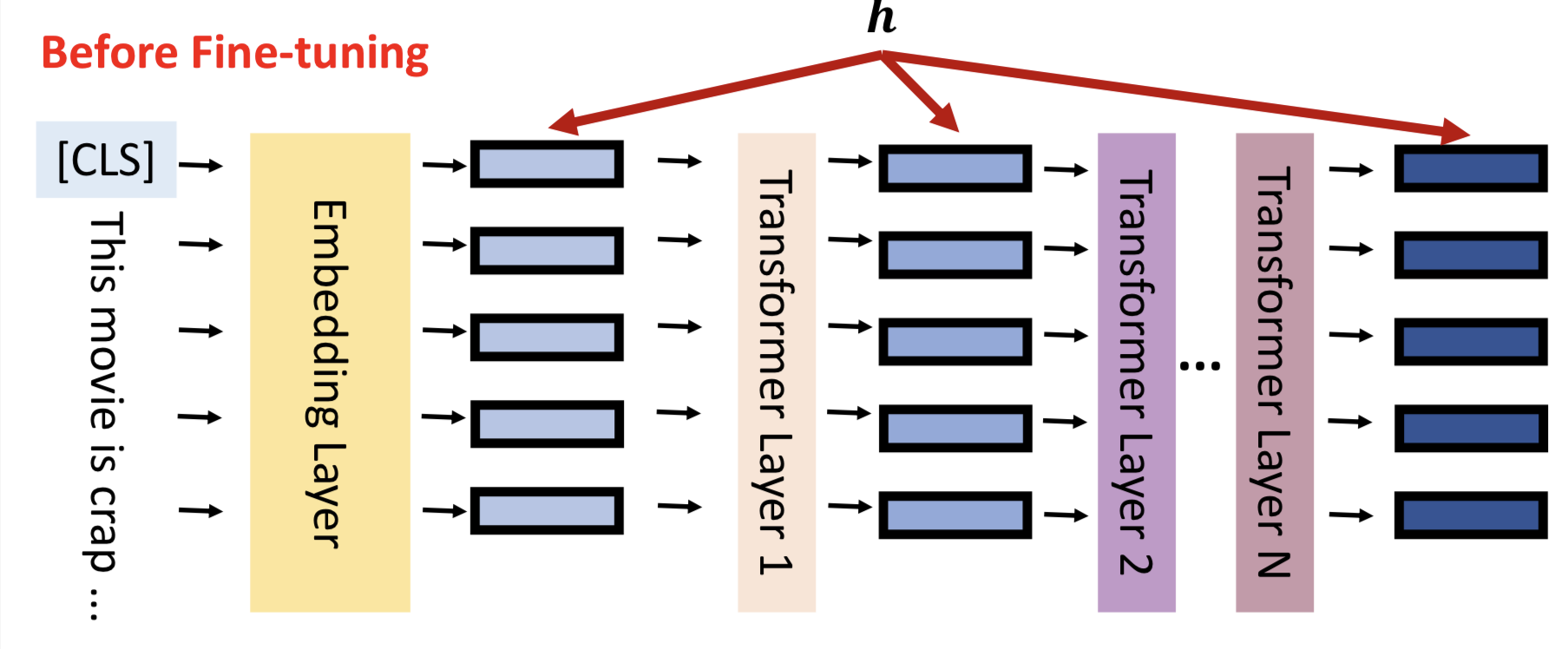
让我们回到模型微调的真实含义，如图所示，h表示每一层隐藏层的输出。

模型微调就是通过数据更新隐藏层的输出结果，更好的拟合输入数据的分布，对下游任务有更佳的表现，我们将隐藏层输出成为hidden representation(h)。
模型微调的结果就是更新hidden representation，用数学语言可以表示为：
h’ = h + 𝚫h
接下来介绍4种不同的方法，通过减少模型参数更新的数量，高效的更新𝚫h。

Adapter方法

Adapter方法通常是在网络模型中增加小型的模型块，通过冻结LLM的参数，仅更新Adapter模块的方式进行模型微调。

如图所示，Adapter应用在Transformer的结构中，在Multi-headed attention和Feed-forward网路层后紧接Adapter子模块，模型训练的时候冻结Transformer的参数，仅更新Adapter的参数。

LoRA方法

LoRA提出的想法是，既然LLM可以泛化用于不同的NLP任务，那么说明不同的任务有不同的神经元来处理，我们只要针对下游任务找到合适的那一批神经元，并对他们的权重进行强化，那么对下游任务也有显著的效果。

LoRA方法假设下游任务只需要低秩矩阵就可以找到大模型中对应的权重，然后仅更新小部分的模型参数，就可以在下游任务中表现不错。

如图所示，LoRA将𝚫h的计算方式更改为两个低秩矩阵的乘法，r表示矩阵秩的大小。那么模型的更新过程可以用数学方式表示为：
W= W + 𝚫W = W + BA, r << min(d_ffw, d_model)

Prefix Learning方法

Prefix Learning方法就是在网络层中，将网络层中扩展可训练的前缀。

这里以Self-Attention为例，先回忆一下Self-Attention的结构。
Self-Attention的数学表示为：
$softmax(\frac{QK^T}{\sqrt{d_k}} V)$
首先初始化W_k, W_q, W_v参数，通过 $q_1=x_1*W_q, k_1=x_1* W_k, v_1=x_1 * W_v$ 的方式得到QKV矩阵；
通过 $\alpha1,1 = q_1 * k_1, \alpha1,2=q_1 * k_2…$ 的方式获取𝛼矩阵；
通过 $z1,1=softmax(\alpha1,1 * v1)…$ 的方式得到x1对其他token的注意力
最后累加计算得出 $x'_1$ 的结果，如此循环计算下一个时刻输出。

PreFix Tuning的做法是对self-attention增加一部分参数，计算𝚫h的结果。
如图所示，增加了3个参数量，模型训练的时候只更新这3个用到的的参数。

Soft Prompt方法

Soft Prompt的做法比较简单，直接在Embedding输出，插入一部分Prefix embedding信息。

Soft Prompt的简化版本是直接在input sequence句首插入文本。

小结

了解4种PEFT的方法后，可以发现PEFT有非常多的好处。
首先，PEFT可以极大的降低finetune的参数量。

如图所示，Adapter训练参数之占模型的5%，LoRa、Prefix Tuning和Soft Prompt的训练参数甚至小于0.1%。
其次，由于训练参数的减少，PEFT更不容易造成模型的过拟合，某种意义也是一种Dropout方法。
最后，由于需要更新的参数少，基础模型在小数据集上有不错的表现。

实践

我们以最受欢迎的LoRA为例，搭建一个简易的demo理解如何使用LoRA微调模型。
Demo的有2个不同分布的数据，分别是均匀分布和高斯分布；然后构造3层的ReLU-MLP对均匀分布数据进行训练；最后通过LoRA的对高斯分布数据进行微调。

首先是构造数据，分别生成均匀分布和高斯分布的数据集，lable范围都是{-1,1}。

import numpy as np
import torch
import matplotlib.pyplot as plt
from torch.utils.data import TensorDataset, DataLoader
import random
from collections import OrderedDict
import math
import torch.nn.functional as F
random.seed(42)

def generate_uniform_sphere(n, d):
    normal_data = np.random.normal(loc=0.0, scale=1.0, size=[n, d])
    lambdas = np.sqrt((normal_data * normal_data).sum(axis=1))
    data = np.sqrt(d) * normal_data / lambdas[:, np.newaxis]
    return data

# data type could be "uniform" or "gaussian"
def data_generator(data_type='uniform', inp_dims=100, sample_size=10000):
    if data_type == 'uniform':
        data = generate_uniform_sphere(sample_size, inp_dims)
    elif data_type == 'gaussian':
        var = 1.0 / inp_dims
        data = np.random.normal(loc=0.0, scale=var, size=[sample_size, inp_dims])

    labels = np.sign(np.mean(data, -1))
    for i in range(sample_size):
        if labels[i] == 0:
            labels[i] = 1
    return data, labels

第二步，构造3层的MLP网络模型，ReLU作为激活函数。

class ReluNN(torch.nn.Module):
    def __init__(self, inp_dims, h_dims, out_dims=1):
        super(ReluNN, self).__init__()
        self.inp_dims = inp_dims
        self.h_dims = h_dims
        self.out_dims = out_dims
        
        # build model
        self.layer1 = torch.nn.Linear(self.inp_dims, self.h_dims)
        self.layer2 = torch.nn.Linear(self.h_dims, self.h_dims)
        self.last_layer = torch.nn.Linear(self.h_dims, self.out_dims, bias=False)

    def forward(self, x: torch.Tensor) -> torch.Tensor:
        x = torch.flatten(x, start_dim=1)
        x = self.layer1(x)
        x = torch.nn.ReLU()(x)
        x = self.layer2(x)
        x = torch.nn.ReLU()(x)
        x = self.last_layer(x)
        return x

def calc_loss(logits, labels):
    return torch.mean(torch.log(1 + torch.exp(-1 * torch.mul(labels.float(), logits.T))))

def evaluate(labels, loss=None, output=None, iter=0, training_time=True):
    correct_label_count = 0
    for i in range(len(output)):
        if (output[i] * labels[i] > 0).item():
            correct_label_count += 1
    if training_time:
        print('Iteration: ', iter, ' Loss: ', loss, ' Correct label: ', correct_label_count, '/', len(output))
    else:
        print('Correct label:  ', correct_label_count, '/', len(output), '， Accuracy: ', correct_label_count / len(output))

第三步，开始训练均匀分布数据。

# input dimensions
inp_dims = 16
# hidden dimensions in our model
h_dims = 32
# training sample size
n_train = 2000
# starting learning rate (I didn't end up using any learning rate scheduler. So this will be constant. )
starting_lr = 1e-4
batch_size = 256

# generate data and build pytorch data pipline using TensorDataset module
data_train, labels_train = data_generator(data_type="uniform", inp_dims=inp_dims, sample_size=n_train)
dataset = TensorDataset(torch.Tensor(data_train), torch.Tensor(labels_train))
loader = DataLoader(dataset, batch_size=batch_size, drop_last=True)

# Build the model and define optimiser
model = ReluNN(inp_dims, h_dims)
optimizer = torch.optim.Adam(model.parameters(), lr=starting_lr)

# ---------------------
# Training loop here
# ---------------------

its = 0
epochs = 400
print_freq = 200

for epoch in range(epochs):
    for batch_data, batch_labels in loader:
        optimizer.zero_grad()
        output = model(batch_data)
        loss = calc_loss(output, batch_labels)
        loss.backward()
        optimizer.step()
        
        if its % print_freq == 0:
            correct_labels = evaluate(labels=batch_labels, loss=loss.detach().numpy(), 
                                      output=output, iter=its, training_time=True)

        its += 1

获取训练输出结果：

Iteration:  0  Loss:  0.6975772  Correct label:  126 / 256
Iteration:  200  Loss:  0.6508794  Correct label:  164 / 256
Iteration:  400  Loss:  0.52307904  Correct label:  215 / 256
Iteration:  600  Loss:  0.34722215  Correct label:  240 / 256
Iteration:  800  Loss:  0.21760023  Correct label:  251 / 256
Iteration:  1000  Loss:  0.19394015  Correct label:  241 / 256
Iteration:  1200  Loss:  0.124890685  Correct label:  250 / 256
Iteration:  1400  Loss:  0.10578571  Correct label:  250 / 256
Iteration:  1600  Loss:  0.07651  Correct label:  252 / 256
Iteration:  1800  Loss:  0.05156578  Correct label:  256 / 256
Iteration:  2000  Loss:  0.045886587  Correct label:  256 / 256
Iteration:  2200  Loss:  0.04692286  Correct label:  256 / 256
Iteration:  2400  Loss:  0.06285152  Correct label:  254 / 256
Iteration:  2600  Loss:  0.03973126  Correct label:  254 / 256

在均匀分布和高斯分布测试集分别进行测试：

print('-------------------------------------------------')
print('Test model performance on uniformly-distributed data (the data we trained our model on)')
data_test, labels_test = data_generator(data_type="uniform", inp_dims=inp_dims, sample_size=1024)
data_test = torch.Tensor(data_test)
labels_test = torch.Tensor(labels_test)

output = model(data_test)
correct_labels = evaluate(labels=labels_test, loss=0.0, output=output, iter=0, training_time=False)

print('-------------------------------------------------')
print('Test model performance on normally-distributed data')
data_test, labels_test = data_generator(data_type="gaussian", inp_dims=inp_dims, sample_size=1024)
data_test = torch.Tensor(data_test)
labels_test = torch.Tensor(labels_test)

output = model(data_test)
correct_labels = evaluate(labels=labels_test, loss=0.0, output=output, iter=0, training_time=False)
print('-------------------------------------------------')

获得输出结果为，均匀分布表现远高于高斯分布，这是理所当然的。

-------------------------------------------------
Test model performance on uniformly-distributed data (the data we trained our model on)
Correct label:   1007 / 1024 ， Accuracy:  0.9833984375
-------------------------------------------------
Test model performance on normally-distributed data
Correct label:   832 / 1024 ， Accuracy:  0.8125
-------------------------------------------------

第四步，实现LoRA改造网络模型，LoRA代码实现来自https://github.com/microsoft/LoRA/tree/main。

class LoRALinear(torch.nn.Linear):
    def __init__(
        self, 
        layer: torch.nn.Linear, 
        r: int, 
        lora_alpha: float, 
        in_features: int, 
        out_features: int,
        **kwargs, 
    ):
        torch.nn.Linear.__init__(self, in_features, out_features, **kwargs)

        # trainable parameters
        self.weight = layer.weight
        
        self.r = r
        if self.r > 0:
            # lora_A matrix has shape [number of ranks, number of input features]
            self.lora_A = torch.nn.Parameter(self.weight.new_zeros((in_features, r)))
            
            # lora_A matrix has shape [number of output features, number of ranks]
            self.lora_B = torch.nn.Parameter(self.weight.new_zeros((r, out_features)))
            
            self.scaling = lora_alpha / r
            
            # Freezing the pre-trained weight matrix
            self.weight.requires_grad = False
            
        self.reset_parameters()
        
    def reset_parameters(self):
        if hasattr(self, 'lora_A'):
            torch.nn.init.kaiming_uniform_(self.lora_A, a=math.sqrt(5))
            torch.nn.init.zeros_(self.lora_B)

    def forward(self, x: torch.Tensor):
        if self.r > 0:
            result = F.linear(x, self.weight, bias=self.bias)            
            result += (x @ self.lora_A @ self.lora_B) * self.scaling
            return result
        else:
            return F.linear(x, self.weight, bias=self.bias)

改造第二层网络层：

ranks = 2
l_alpha = 1.0

# wrap the second layer of the model
lora_layer2 = LoRALinear(model.layer2, r=ranks, lora_alpha=l_alpha, in_features=h_dims, out_features=h_dims)

开始进行微调训练：

# new pipline that contains data generated from Gaussian distribution
ft_data_train, ft_labels_train = data_generator(data_type="gaussian", inp_dims=inp_dims, sample_size=n_train)
ft_data_test, ft_labels_test = data_generator(data_type="gaussian", inp_dims=inp_dims, sample_size=n_train)
dataset = TensorDataset(torch.Tensor(ft_data_train), torch.Tensor(ft_labels_train))
ft_loader = DataLoader(dataset, batch_size=batch_size, drop_last=False)

# Adam now takes the 160 trainable LoRA parameters 
starting_lr = 1e-3
optimizer = torch.optim.Adam(lora_layer2.parameters(), lr=starting_lr)

# ---------------------
# Training starts again
# ---------------------

its = 0
epochs = 400
print_freq = 200

for epoch in range(epochs):
    for batch_data, batch_labels in ft_loader:
        optimizer.zero_grad()
        
        x = model.layer1(batch_data)
        x = torch.nn.ReLU()(x)
        # ---this is the new layer---
        x = lora_layer2(x)
        # ---------------------------
        x = torch.nn.ReLU()(x)
        output = model.last_layer(x)
        
        loss = calc_loss(output, batch_labels)
        loss.backward()
        optimizer.step()
        
        if its % print_freq == 0:
            correct_labels = evaluate(labels=batch_labels, loss=loss.detach().numpy(), 
                                      output=output, iter=its, training_time=True)

        its += 1

微调输出结果为：

Iteration:  0  Loss:  0.41668275  Correct label:  194 / 256
Iteration:  200  Loss:  0.34483075  Correct label:  249 / 256
Iteration:  400  Loss:  0.28130627  Correct label:  247 / 256
Iteration:  600  Loss:  0.18952605  Correct label:  249 / 256
Iteration:  800  Loss:  0.14345655  Correct label:  249 / 256
Iteration:  1000  Loss:  0.117519796  Correct label:  250 / 256
Iteration:  1200  Loss:  0.100797206  Correct label:  251 / 256
Iteration:  1400  Loss:  0.08887711  Correct label:  252 / 256
Iteration:  1600  Loss:  0.07975915  Correct label:  253 / 256
Iteration:  1800  Loss:  0.07250729  Correct label:  253 / 256
Iteration:  2000  Loss:  0.06658038  Correct label:  253 / 256
Iteration:  2200  Loss:  0.061622016  Correct label:  254 / 256
Iteration:  2400  Loss:  0.057407677  Correct label:  254 / 256
Iteration:  2600  Loss:  0.05379172  Correct label:  254 / 256
Iteration:  2800  Loss:  0.050651148  Correct label:  254 / 256
Iteration:  3000  Loss:  0.04789203  Correct label:  255 / 256

最后一步，再次测试高斯分布的数据集。

data_test, labels_test = data_generator(data_type="gaussian", inp_dims=inp_dims, sample_size=1024)
data_test = torch.Tensor(data_test)
labels_test = torch.Tensor(labels_test)

x = model.layer1(data_test)
x = torch.nn.ReLU()(x)
# ---this is the new layer---
x = lora_layer2(x)
# ---------------------------
x = torch.nn.ReLU()(x)
output = model.last_layer(x)
correct_labels = evaluate(labels=labels_test, loss=0.0, output=output, iter=0, training_time=False)

输出结果为：

Correct label:   1011 / 1024 ， Accuracy:  0.9873046875

微调效果很明显，准确率从81.2%提升到98.7%。最后再计算LoRA微调的参数量大小。

def count_parameters(model):
    return sum(p.numel() for p in model.parameters() if p.requires_grad)
    
print("Original second layer parameters: ", count_parameters(original_layer2))
print("LoRA layer parameters: ", count_parameters(lora_layer2))

输出结果为：

Original second layer parameters:  1056
LoRA layer parameters:  160

通过实验结果发现，原始模型参数量1056，LoRA参数量160，仅为原来的1/10，但是训练效果从81.2%提升到98.7%。

总结

如果对网络层每一层都要重新实现LoRA的方法，是比较复杂的，推荐使用HuggingFace的封装库peft，覆盖基本的网络模型。

共用基础LLM是未来的趋势，如果需要快速适应特殊的任务，只需要训练LoRA的参数即可，大大降低了GPU的使用量；
当不同任务的切换时，只需要切换不同的LoRA参数；

参考

Houlsby, Neil, et al. “Parameter-efficient transfer learning for NLP.” International Conference on Machine Learning. PMLR, 2019.
Hu, Edward J., et al. “LoRA: Low-Rank Adaptation of Large Language Models.” International Conference on Learning Representations. 2021.
The Power of Scale for Parameter-Efficient Prompt Tuning. Proceedings of the 2021 Conference on Empirical Methods in Natural Language Processing. 2021