文章目录
- 1、实验内容
- 2、实验设计(略)
- 3、实验环境及实验数据集
- 四、实验过程及结果
- 4.1 Harris角点检测器寻找关键点
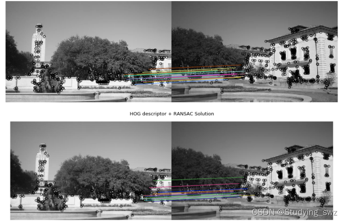
- 4.2 构建描述算子来描述图中的每个关键点,比较两幅图像的两组描述子,并进行匹配。
- 4.3 根据一组匹配关键点,使用最小二乘法进行仿射变换矩阵的计算
- 4.4 使用RANSAC计算一个更加稳定的仿射变换的矩阵,然后将第二幅图变换过来并覆盖在第一幅图上,形成一个全景
- 4.5 实现不同的描述子HOG,得到不同的拼接结果
1、实验内容
实验题目:Implement Panorama Stitching with Harris corner detector, RANSAC and HOG descriptor.
实验步骤:
- 1.使用Harris焦点检测器寻找关键点。
- 2.构建描述算子来描述图中的每个关键点,比较两幅图像的两组描述子,并进行匹配。
- 3.根据一组匹配关键点,使用最小二乘法进行仿射变换矩阵的计算。
- 4.使用RANSAC计算一个更加稳定的仿射变换的矩阵,然后将第二幅图变换过来并覆盖在第一幅图上,形成一个全景。
- 5.实现不同的描述子,并得到不同的拼接结果。
2、实验设计(略)
3、实验环境及实验数据集
实验环境:
- Windows10的操作系统、anaconda3、python3.6、jupyter notebook。
数据集:
- 任务给出的原图片以及处理结果后的图片,如image1.jpg、image2.jpg、solution_harris.png等等。
四、实验过程及结果
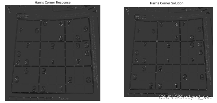
4.1 Harris角点检测器寻找关键点
结果展示:
实现代码:
1.def harris_corners(img, window_size=3, k=0.04):
2. """
3. Compute Harris corner response map. Follow the math equation
4. R=Det(M)-k(Trace(M)^2).
5.
6. Hint:
7.     You may use the function scipy.ndimage.filters.convolve,
8.     which is already imported above.
9.
10. Args:
11.     img: Grayscale image of shape (H, W)
12.     window_size: size of the window function
13.     k: sensitivity parameter
14.
15. Returns:
16.     response: Harris response image of shape (H, W)
17. """
18.
19. H, W = img.shape
20. window = np.ones((window_size, window_size))
21.
22. response = np.zeros((H, W))
23.
24. dx = filters.sobel_v(img)
25. dy = filters.sobel_h(img)
26.
27. ### YOUR CODE HERE
28. Ix2 = np.multiply(dx,dx)
29. Iy2 = np.multiply(dy,dy)
30. IxIy = np.multiply(dx,dy)
31.
32. #高斯加权
33. A = convolve(Ix2,window)
34. B = convolve(Iy2,window)
35. C = convolve(IxIy,window)
36.
37. detM = np.multiply(A, B) - np.multiply(C, C)
38. traceM = A + B
39.
40. response = detM - k * np.square(traceM)
41. ### END YOUR CODE
42.
 return response
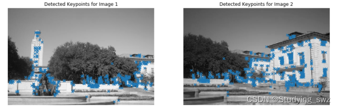
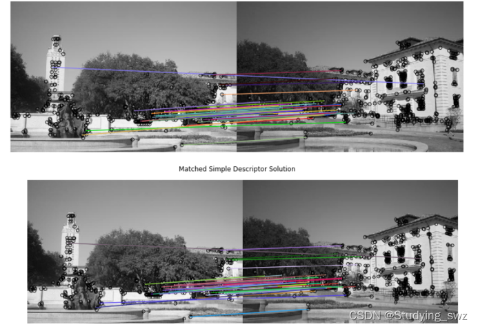
4.2 构建描述算子来描述图中的每个关键点,比较两幅图像的两组描述子,并进行匹配。
结果展示:
实现代码:
构建描述算子
1.def simple_descriptor(patch):
2. """
3. Describe the patch by normalizing the image values into a standard
4. normal distribution (having mean of 0 and standard deviation of 1)
5. and then flattening into a 1D array.
6.
7. The normalization will make the descriptor more robust to change
8. in lighting condition.
9.
10. Hint:
11.     If a denominator is zero, divide by 1 instead.
12.
13. Args:
14.     patch: grayscale image patch of shape (H, W)
15.
16. Returns:
17.     feature: 1D array of shape (H * W)
18. """
19. feature = []
20. ### YOUR CODE HERE
21. mean = np.mean(patch)
22. sigma = np.std(patch)
23. if sigma == 0.0:
24.     sigma = 1
25. #均值0,标准差为1
26. normalized = (patch - mean) / sigma
27. #生成一维特征向量
28. feature = normalized.flatten()
29. ### END YOUR CODE
30. return feature
根据描述子进行匹配
1.#注意,这里引入了heapq堆排列模块算法
2.import heapq
3.def match_descriptors(desc1, desc2, threshold=0.5):
4.    """
5.    Match the feature descriptors by finding distances between them. A match is formed
6.    when the distance to the closest vector is much smaller than the distance to the
7.    second-closest, that is, the ratio of the distances should be smaller
8.    than the threshold. Return the matches as pairs of vector indices.
9.
10.    Hint:
11.        The Numpy functions np.sort, np.argmin, np.asarray might be useful
12.
13.    Args:
14.        desc1: an array of shape (M, P) holding descriptors of size P about M keypoints
15.        desc2: an array of shape (N, P) holding descriptors of size P about N keypoints
16.
17.    Returns:
18.        matches: an array of shape (Q, 2) where each row holds the indices of one pair
19.        of matching descriptors
20.    """
21.    matches = []
22.
23.    N = desc1.shape[0]
24.    dists = cdist(desc1, desc2)
25.
26.    ### YOUR CODE HERE
27.    for i in range(N):
28.        #找到最近的两个值
29.        min2 = heapq.nsmallest(2, dists[i,:])
30.        #保证最小的和第二小的有一定的距离
31.        if min2[0] / min2[1] < threshold:
32.            matches.append([i, np.argmin(dists[i,:])])
33.    matches = np.asarray(matches)
34.    ### END YOUR CODE
35.
36.    return matches
4.3 根据一组匹配关键点,使用最小二乘法进行仿射变换矩阵的计算
实验结果:

实验代码:
1.def fit_affine_matrix(p1, p2):
2. """ Fit affine matrix such that p2 * H = p1
3.
4. Hint:
5.     You can use np.linalg.lstsq function to solve the problem.
6.
7. Args:
8.     p1: an array of shape (M, P)
9.     p2: an array of shape (M, P)
10.
11. Return:
12.     H: a matrix of shape (P, P) that transform p2 to p1.
13. """
14.
15. assert (p1.shape[0] == p2.shape[0]),\
16.     'Different number of points in p1 and p2'
17. p1 = pad(p1)
18. p2 = pad(p2)
19.
20. ### YOUR CODE HERE
21. #仿射变换矩阵
22. H, residuals, rank, s = np.linalg.lstsq(p2, p1, rcond=None)
23. ### END YOUR CODE
24.
25. # Sometimes numerical issues cause least-squares to produce the last
26. # column which is not exactly [0, 0, 1]
27. H[:,2] = np.array([0, 0, 1])
28. return H
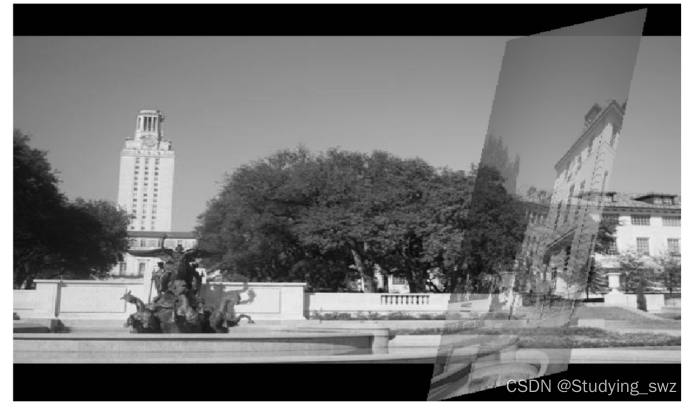
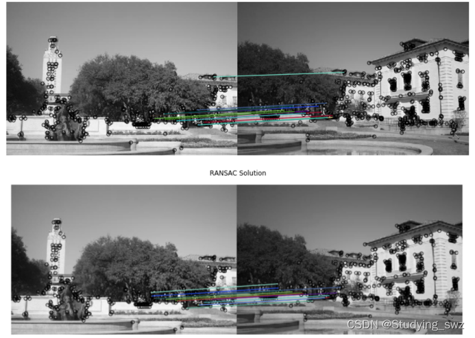
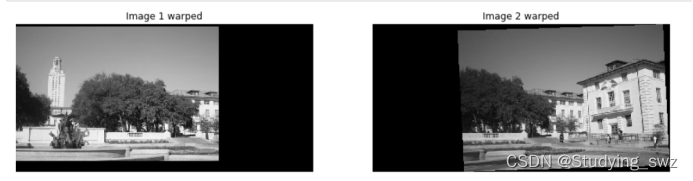
4.4 使用RANSAC计算一个更加稳定的仿射变换的矩阵,然后将第二幅图变换过来并覆盖在第一幅图上,形成一个全景
实验结果:

实验代码:
1.def ransac(keypoints1, keypoints2, matches, n_iters=200, threshold=20):
2. """
3. Use RANSAC to find a robust affine transformation
4.
5.     1. Select random set of matches
6.     2. Compute affine transformation matrix
7.     3. Compute inliers
8.     4. Keep the largest set of inliers
9.     5. Re-compute least-squares estimate on all of the inliers
10.
11. Args:
12.     keypoints1: M1 x 2 matrix, each row is a point
13.     keypoints2: M2 x 2 matrix, each row is a point
14.     matches: N x 2 matrix, each row represents a match
15.         [index of keypoint1, index of keypoint 2]
16.     n_iters: the number of iterations RANSAC will run
17.     threshold: the number of threshold to find inliers
18.
19. Returns:
20.     H: a robust estimation of affine transformation from keypoints2 to
21.     keypoints 1
22. """
23. # Copy matches array, to avoid overwriting it
24. orig_matches = matches.copy()
25. matches = matches.copy()
26.
27. N = matches.shape[0]
28. print(N)
29. n_samples = int(N * 0.2)
30.
31. matched1 = pad(keypoints1[matches[:,0]])
32. matched2 = pad(keypoints2[matches[:,1]])
33.
34. max_inliers = np.zeros(N)
35. n_inliers = 0
36.
37. # RANSAC iteration start
38. ### YOUR CODE HERE
39. for i in range(n_iters):
40.     inliersArr = np.zeros(N)
41.     idx = np.random.choice(N, n_samples, replace=False)
42.     p1 = matched1[idx, :]
43.     p2 = matched2[idx, :]
44.
45.     H, residuals, rank, s = np.linalg.lstsq(p2, p1, rcond=None)
46.     H[:, 2] = np.array([0, 0, 1])
47.
48.     output = np.dot(matched2, H)
49.     inliersArr = np.linalg.norm(output-matched1, axis=1)**2 < threshold
50.     inliersCount = np.sum(inliersArr)
51.
52.     if inliersCount > n_inliers:
53.         max_inliers = inliersArr.copy() #这里需要注意深拷贝和浅拷贝
54.         n_inliers = inliersCount
55.
56. # 迭代完成,拿最大数目的匹配点对进行估计变换矩阵
57. H, residuals, rank, s = np.linalg.lstsq(matched2[max_inliers], matched1[max_inliers], rcond=None)
58. H[:, 2] = np.array([0, 0, 1])
59. ### END YOUR CODE
60. print(H)
61. return H, orig_matches[max_inliers]
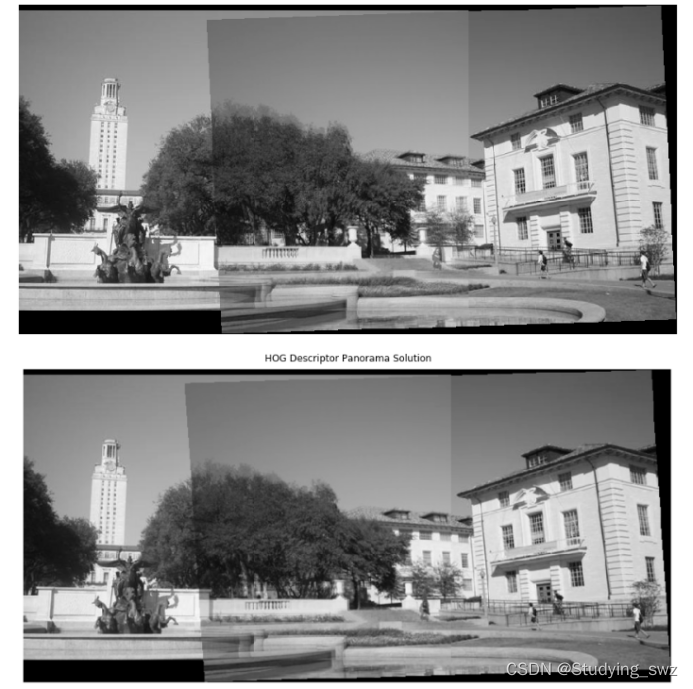
4.5 实现不同的描述子HOG,得到不同的拼接结果
实验结果:

实验代码:
1.def hog_descriptor(patch, pixels_per_cell=(8,8)):
2. """
3. Generating hog descriptor by the following steps:
4.
5. 1. Compute the gradient image in x and y directions (already done for you)
6. 2. Compute gradient histograms for each cell
7. 3. Flatten block of histograms into a 1D feature vector
8.     Here, we treat the entire patch of histograms as our block
9. 4. Normalize flattened block
10.     Normalization makes the descriptor more robust to lighting variations
11.
12. Args:
13.     patch: grayscale image patch of shape (H, W)
14.     pixels_per_cell: size of a cell with shape (M, N)
15.
16. Returns:
17.     block: 1D patch descriptor array of shape ((H*W*n_bins)/(M*N))
18. """
19. assert (patch.shape[0] % pixels_per_cell[0] == 0),\
20.             'Heights of patch and cell do not match'
21. assert (patch.shape[1] % pixels_per_cell[1] == 0),\
22.             'Widths of patch and cell do not match'
23.
24. n_bins = 9
25. degrees_per_bin = 180 // n_bins
26.
27. Gx = filters.sobel_v(patch)
28. Gy = filters.sobel_h(patch)
29.
30. # Unsigned gradients
31. G = np.sqrt(Gx**2 + Gy**2)
32. theta = (np.arctan2(Gy, Gx) * 180 / np.pi) % 180
33.
34. # Group entries of G and theta into cells of shape pixels_per_cell, (M, N)
35. #   G_cells.shape = theta_cells.shape = (H//M, W//N)
36. #   G_cells[0, 0].shape = theta_cells[0, 0].shape = (M, N)
37. G_cells = view_as_blocks(G, block_shape=pixels_per_cell)
38. theta_cells = view_as_blocks(theta, block_shape=pixels_per_cell)
39. rows = G_cells.shape[0]
40. cols = G_cells.shape[1]
41.
42. # For each cell, keep track of gradient histrogram of size n_bins
43. cells = np.zeros((rows, cols, n_bins))
44.
45. # Compute histogram per cell
46. ### YOUR CODE HERE
47. # 首先需要遍历Cell
48. for row in range(rows):
49.     for col in range(cols):
50.         # 遍历cell中的像素
51.         for y in range(pixels_per_cell[0]):
52.             for x in range(pixels_per_cell[1]):
53.                 # 计算该像素的梯度方向(在n_bins个方向中属于第几个区间)
54.                 angle = theta_cells[row,col,y,x]
55.                 order = int(angle) // degrees_per_bin
56.                 if order == 9:
57.                     order = 8
58.                 # 统计该cell中每个方向区间内的强度
59.                 # 累加强度也可以
60.                 cells[row,col,order] += G_cells[row,col,y,x]
61.
62. # 最后做归一化处理,直方图归一化
63. cells = (cells - cells.mean()) / (cells.std())
64. block = cells.reshape(-1) # 一维
65. ### YOUR CODE HERE
66.
67. return block
完整实验见下载连接:
https://download.csdn.net/download/qq_37534947/88222832