最近在团队的OLAP引擎上做了一些SQL编译优化的工作，整理到了语雀上，也顺便发在博客上了。SQL编译优化理论并不复杂，只需要掌握一些关系代数的基础就比较好理解；比较困难的在于reorder算法部分。

基础概念

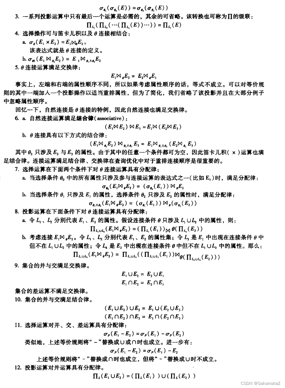
关系代数等价

参考《数据库系统概念》第七版
下面是第六版


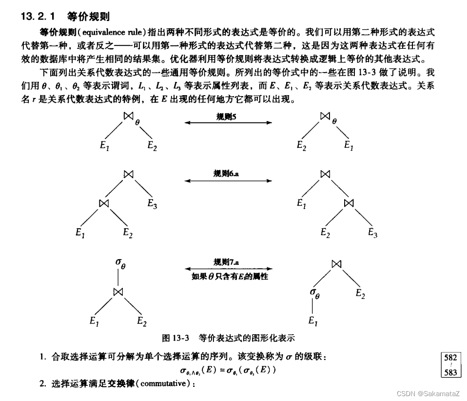
注意自然连接和θ连接的交换律不能用于外连接

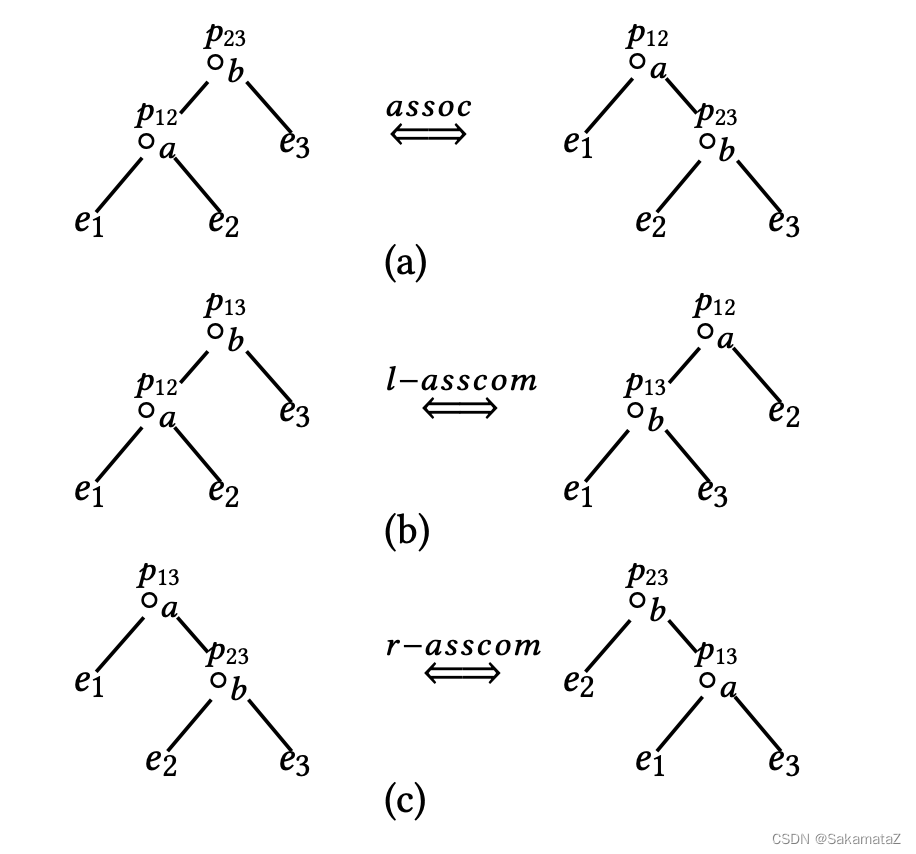
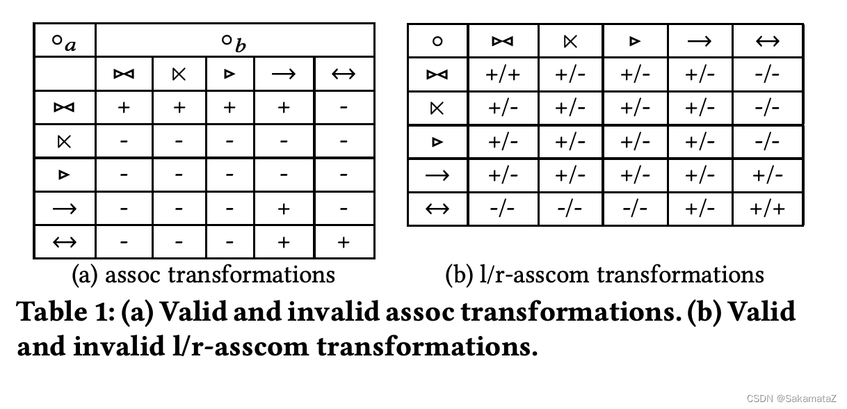
join等价规则

https://www.comp.nus.edu.sg/~chancy/sigmod18-reorder.pdf

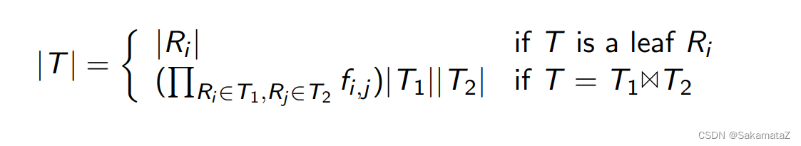
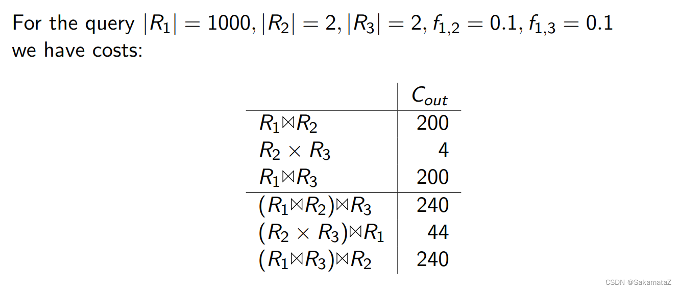
基数

基数（cardinality）表示不同值的数量

、

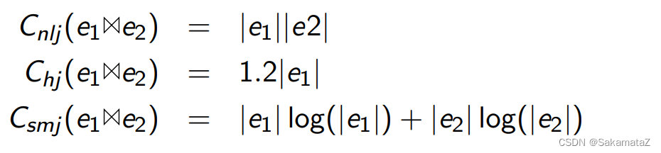
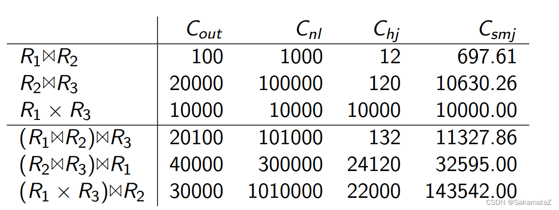
join算法的成本

从上到下依次为嵌套循环连接、hash连接、排序合并连接

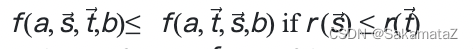
ASI（相邻序列交换）

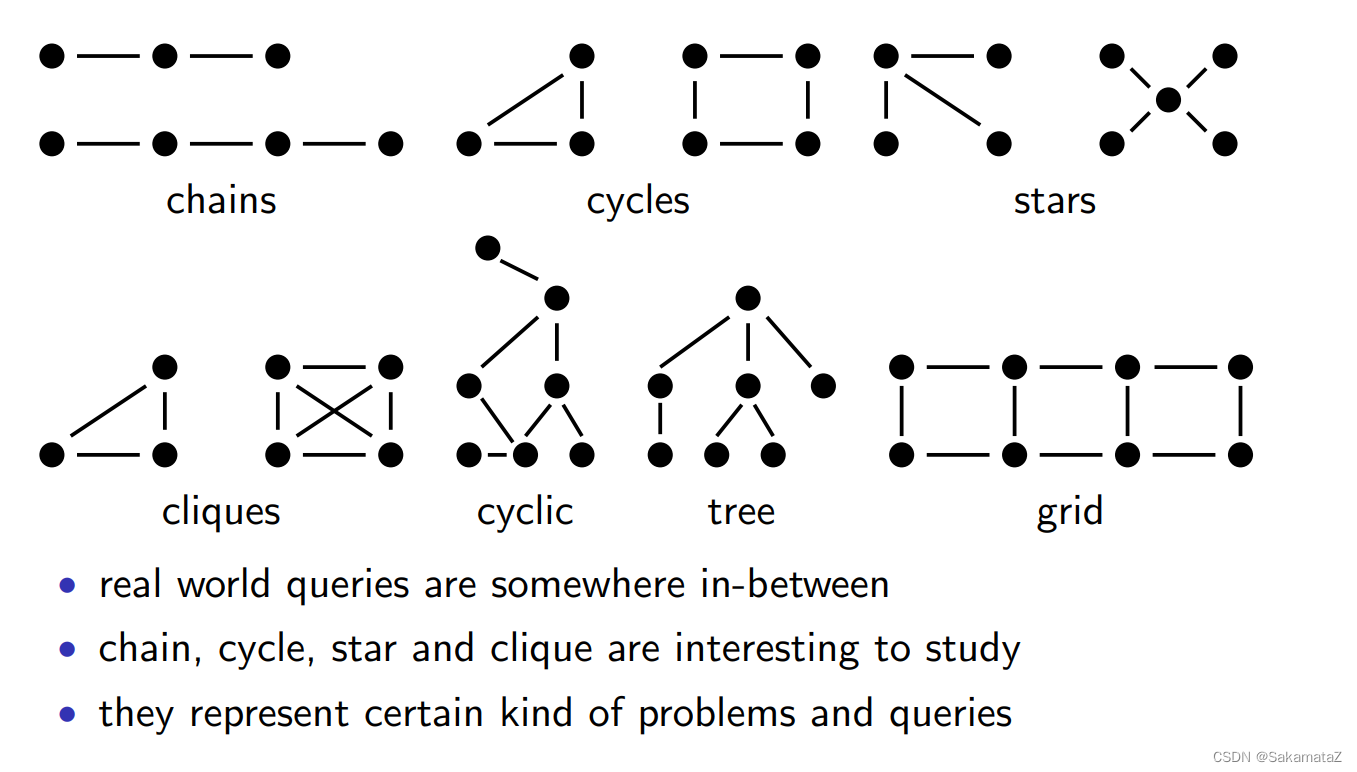
查询问题的分类

按照查询图：chain、cycle、star、clique
按照查询树结构：left-deep、zig-zag、bushy tree
按照join结构：有没有cross product
按照成本函数：有没有ASI属性

连接树的可能数量（搜索空间）

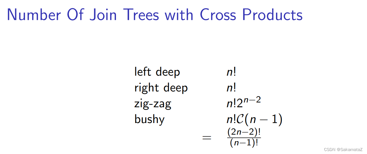
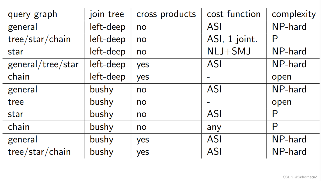
查询图、join树和问题复杂度

Calcite概念

RelNode：plan/subplan
relset：关系表达式等价的plan集合
relsubset ：关系表达式和物理属性等价的plan集合
transformationRule：logical plan变化的规则集合
converterplan：将lp转化为pp的转化规则
RelOptRule ：优化规则
RelOptNode 接口, 它代表的是能被 planner 操作的 expression node
statement：语句
reltrait 关系表达式特征
RelTraitDef 用于定义一类 RelTrait
RelTrait RelTrait是一个表示查询计划特征的抽象类。它用于描述查询计划的一些特性，是对应 TraitDef 的具体实例
Convention 是一种 RelTrait 用于表示 Rel 的调用约定(calling convention)
rexnode 行表达式
schema：逻辑模型
Program：一个SQL查询解析和优化的过程集合，可以将多个子过程组合在一起，以便进行SQL查询的解析和优化

cascade/volcano

volcano是top-down的模块化可剪枝sql优化模型。
volcano生成两个代数模型：logical and the physical algebras 分别优化lp和pp（pp主要选择执行算法）
一个volcano优化器必须提供如下部分：
(1) a set of logical operators,
(2) algebraic transformation rules, possibly with condition code,
(3) a set of algorithms and enforcers,
(4) implementation rules, possibly with condition code,
(5) an ADT “cost” with functions for basic arithmetic and comparison,
(6) an ADT “logical properties,”
(7) an ADT “physical property vector” including comparisons functions (equality and cover),
(8) an applicability function for each algorithm and enforcer,
(9) a cost function for each algorithm and enforcer,
(10) a property function for each operator, algorithm, and enf
volcano使用backward chaining的方式，只探索实际参与更大表达式的子查询和计划。这种方法可以避免对无关的子查询和计划进行搜索，从而提高查询优化的效率。

Calcite volcano递归优化器实现

RuleQueue 是一个优先队列，包含当前所有可行的 RuleMatch，findBestExpr() 时每次循环中我们从中取出优先级最高的并 apply，再根据 apply 的结果更新队列……如此往复，直到满足终止条件。
RuleQueue并没有使用大顶堆，仅仅保存了importance最大的节点。
我们想象我们现在有一组relnode，匹配上了很多RuleMatch，怎么决定先进行哪个match呢？
RuleMatch的importance决定了先进行哪个match，rulematch的importance定义为以下两个中较大的一个：

1. 输入的 RelSubset 的 importance
2. 输出的 RelSubset 的 importance
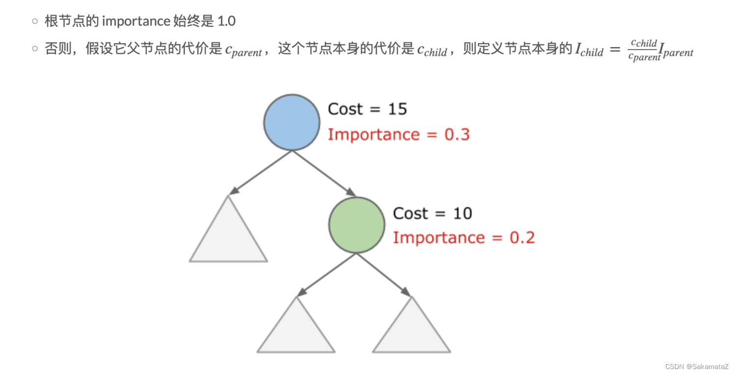
   RelSubset的importance又该如何定义？importance 定义为以下两个中比较大的一个：
   ● 该 RelSubset 本身的真实 importance
   ● 逻辑上相等的（即位于同一个 RelSet 中）任意一个 RelSubset 的真实 importance 除以 2
   真实importance的计算规则如下：
   
   

Join reorder

大部分的算法基于connectivity-heuristic，也就是说，只考虑equl-join

基于连接次序优化的动态规划算法

对于假设所有的连接都是自然连接的n个关系的集合，动态规划算法的复杂度为3^n
归并连接可以产生有序的结果，对于后面的排序可能有用（interesting sort order）。
目前我们用spark的连接算法，这条暂时没用。

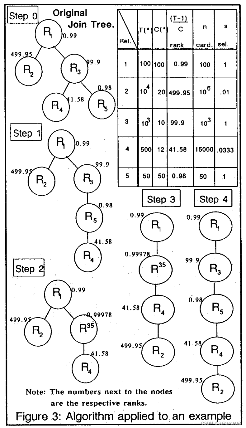
IKKBZ算法

left-deep tree和bushy tree
left-deep tree 左深树
连接运算符的右侧输入都是具体关系，右子树必和左子树的节点之一有共享谓词。

左深树适合一般场景的优化。System R优化器只考虑左深树的优化，时间代价是n！，加入动态规划后，可以在n*2^n时间内找到最佳连接次序。

bushy-tree

适合多路连接和并行优化，但是很复杂。
不引入交叉乘的充要条件在于给定关系的父级必须已经得到。

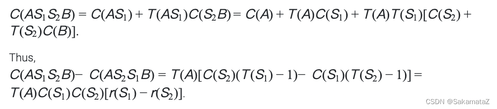
ASI

简单来说就是等价谓词替换原则
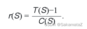
定义rank函数：

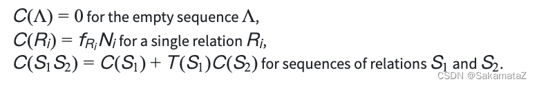
成本函数
谓词的选择性指的是谓词对查询结果的过滤能力
对于join来说可以有如下定义：

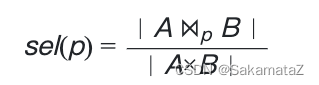
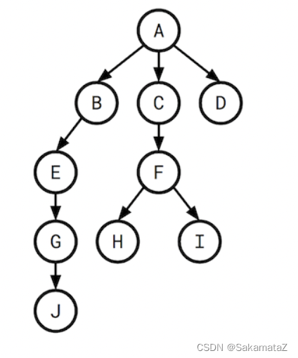
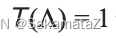
我们将查询图视为一个有根树，我们说H的选择性指的是F和H之间的选择性。
行数和选择性之间则有如下关系（行数*选择性）：

成本函数定义如下：

我们可以根据成本函数定义rank函数：

下面是对于ASI的证明：

归一化

Calcite实践

MultiJoinOptimizeBushyRule

第一部分进行初始化，unusedEdges存放join过滤条件（两个relnode之间）

final MultiJoin multiJoinRel = call.rel(0);
    final RexBuilder rexBuilder = multiJoinRel.getCluster().getRexBuilder();
    final RelBuilder relBuilder = call.builder();
    final RelMetadataQuery mq = call.getMetadataQuery();

    final LoptMultiJoin multiJoin = new LoptMultiJoin(multiJoinRel);

    final List<Vertex> vertexes = new ArrayList<>();
    int x = 0;
    for (int i = 0; i < multiJoin.getNumJoinFactors(); i++) {
      final RelNode rel = multiJoin.getJoinFactor(i);
      double cost = mq.getRowCount(rel);
      vertexes.add(new LeafVertex(i, rel, cost, x));
      x += rel.getRowType().getFieldCount();
    }
    assert x == multiJoin.getNumTotalFields();

    final List<Edge> unusedEdges = new ArrayList<>();
    for (RexNode node : multiJoin.getJoinFilters()) {
      unusedEdges.add(multiJoin.createEdge(node));
    }

第二步选出成本（此处就是行数）差异最大的过滤条件
选一个行数较小的vertex作为majorFactor，另一个作为minorFactor

    // Comparator that chooses the best edge. A "good edge" is one that has
    // a large difference in the number of rows on LHS and RHS.
    final Comparator<LoptMultiJoin.Edge> edgeComparator =
        new Comparator<LoptMultiJoin.Edge>() {
          @Override public int compare(LoptMultiJoin.Edge e0, LoptMultiJoin.Edge e1) {
            return Double.compare(rowCountDiff(e0), rowCountDiff(e1));
          }

          private double rowCountDiff(LoptMultiJoin.Edge edge) {
            assert edge.factors.cardinality() == 2 : edge.factors;
            final int factor0 = edge.factors.nextSetBit(0);
            final int factor1 = edge.factors.nextSetBit(factor0 + 1);
            return Math.abs(vertexes.get(factor0).cost
                - vertexes.get(factor1).cost);
          }
        };

    final List<Edge> usedEdges = new ArrayList<>();
    for (;;) {
      final int edgeOrdinal = chooseBestEdge(unusedEdges, edgeComparator);
      if (pw != null) {
        trace(vertexes, unusedEdges, usedEdges, edgeOrdinal, pw);
      }
      final int[] factors;
      if (edgeOrdinal == -1) {
        // No more edges. Are there any un-joined vertexes?
        final Vertex lastVertex = Util.last(vertexes);
        final int z = lastVertex.factors.previousClearBit(lastVertex.id - 1);
        if (z < 0) {
          break;
        }
        factors = new int[] {z, lastVertex.id};
      } else {
        final LoptMultiJoin.Edge bestEdge = unusedEdges.get(edgeOrdinal);

        // For now, assume that the edge is between precisely two factors.
        // 1-factor conditions have probably been pushed down,
        // and 3-or-more-factor conditions are advanced. (TODO:)
        // Therefore, for now, the factors that are merged are exactly the
        // factors on this edge.
        assert bestEdge.factors.cardinality() == 2;
        factors = bestEdge.factors.toArray();
      }
      
      // Determine which factor is to be on the LHS of the join.
      final int majorFactor;
      final int minorFactor;
      if (vertexes.get(factors[0]).cost <= vertexes.get(factors[1]).cost) {
        majorFactor = factors[0];
        minorFactor = factors[1];
      } else {
        majorFactor = factors[1];
        minorFactor = factors[0];
      }
      final Vertex majorVertex = vertexes.get(majorFactor);
      final Vertex minorVertex = vertexes.get(minorFactor);

遍历unusedEdges，加入newFactors，对之前选出的majorVertex和minorVertex进行归一化并且加入vertexes

      // Find the join conditions. All conditions whose factors are now all in
      // the join can now be used.
      final int v = vertexes.size();
      final ImmutableBitSet newFactors =
          majorVertex.factors
              .rebuild()
              .addAll(minorVertex.factors)
              .set(v)
              .build();

      final List<RexNode> conditions = new ArrayList<>();
      final Iterator<LoptMultiJoin.Edge> edgeIterator = unusedEdges.iterator();
      while (edgeIterator.hasNext()) {
        LoptMultiJoin.Edge edge = edgeIterator.next();
        if (newFactors.contains(edge.factors)) {
          conditions.add(edge.condition);
          edgeIterator.remove();
          usedEdges.add(edge);
        }
      }
      double cost =
        majorVertex.cost
        * minorVertex.cost
        * RelMdUtil.guessSelectivity(
            RexUtil.composeConjunction(rexBuilder, conditions));
      final Vertex newVertex =
          new JoinVertex(v, majorFactor, minorFactor, newFactors,
              cost, ImmutableList.copyOf(conditions));
      vertexes.add(newVertex);

归一化之后进行选择性的重新计算，之后进入下一轮

// Re-compute selectivity of edges above the one just chosen.
      // Suppose that we just chose the edge between "product" (10k rows) and
      // "product_class" (10 rows).
      // Both of those vertices are now replaced by a new vertex "P-PC".
      // This vertex has fewer rows (1k rows) -- a fact that is critical to
      // decisions made later. (Hence "greedy" algorithm not "simple".)
      // The adjacent edges are modified.
      final ImmutableBitSet merged =
          ImmutableBitSet.of(minorFactor, majorFactor);
      for (int i = 0; i < unusedEdges.size(); i++) {
        final LoptMultiJoin.Edge edge = unusedEdges.get(i);
        if (edge.factors.intersects(merged)) {
          ImmutableBitSet newEdgeFactors =
              edge.factors
                  .rebuild()
                  .removeAll(newFactors)
                  .set(v)
                  .build();
          assert newEdgeFactors.cardinality() == 2;
          final LoptMultiJoin.Edge newEdge =
              new LoptMultiJoin.Edge(edge.condition, newEdgeFactors,
                  edge.columns);
          unusedEdges.set(i, newEdge);
        }
      }

最后一段，根据新的vertexes次序建立relnode节点

// We have a winner!
List<Pair<RelNode, TargetMapping>> relNodes = new ArrayList<>();
for (Vertex vertex : vertexes) {
  if (vertex instanceof LeafVertex) {
    LeafVertex leafVertex = (LeafVertex) vertex;
    final Mappings.TargetMapping mapping =
        Mappings.offsetSource(
            Mappings.createIdentity(
                leafVertex.rel.getRowType().getFieldCount()),
            leafVertex.fieldOffset,
            multiJoin.getNumTotalFields());
    relNodes.add(Pair.of(leafVertex.rel, mapping));
  } else {
    JoinVertex joinVertex = (JoinVertex) vertex;
    final Pair<RelNode, Mappings.TargetMapping> leftPair =
        relNodes.get(joinVertex.leftFactor);
    RelNode left = leftPair.left;
    final Mappings.TargetMapping leftMapping = leftPair.right;
    final Pair<RelNode, Mappings.TargetMapping> rightPair =
        relNodes.get(joinVertex.rightFactor);
    RelNode right = rightPair.left;
    final Mappings.TargetMapping rightMapping = rightPair.right;
    final Mappings.TargetMapping mapping =
        Mappings.merge(leftMapping,
            Mappings.offsetTarget(rightMapping,
                left.getRowType().getFieldCount()));
    if (pw != null) {
      pw.println("left: " + leftMapping);
      pw.println("right: " + rightMapping);
      pw.println("combined: " + mapping);
      pw.println();
    }
    final RexVisitor<RexNode> shuttle =
        new RexPermuteInputsShuttle(mapping, left, right);
    final RexNode condition =
        RexUtil.composeConjunction(rexBuilder, joinVertex.conditions);

    final RelNode join = relBuilder.push(left)
        .push(right)
        .join(JoinRelType.INNER, condition.accept(shuttle))
        .build();
    relNodes.add(Pair.of(join, mapping));
  }
  if (pw != null) {
    pw.println(Util.last(relNodes));
  }

Join 算法选择

关联子查询优化

我们将连接外部查询和子查询的算子叫做CorrelatedJoin(也被称之为lateral join, dependent join、apply算子等等。它的左子树我们称之为外部查询(input)，右子树称之为子查询(subquery)。

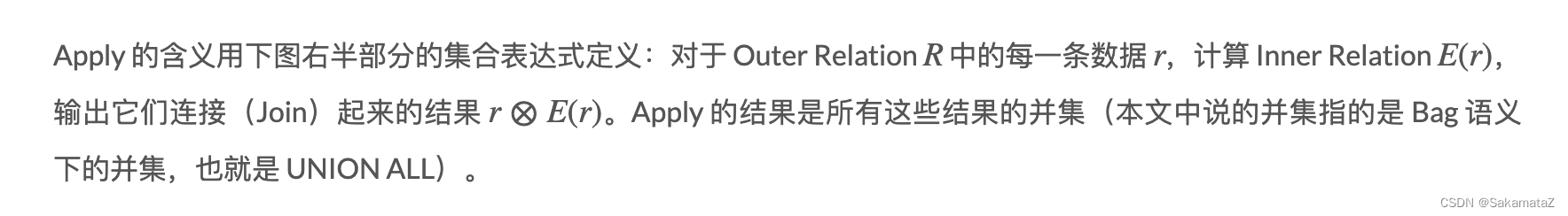
注：bag语义，允许元素重复出现，和set语义正交

为什么要消除关联子查询？

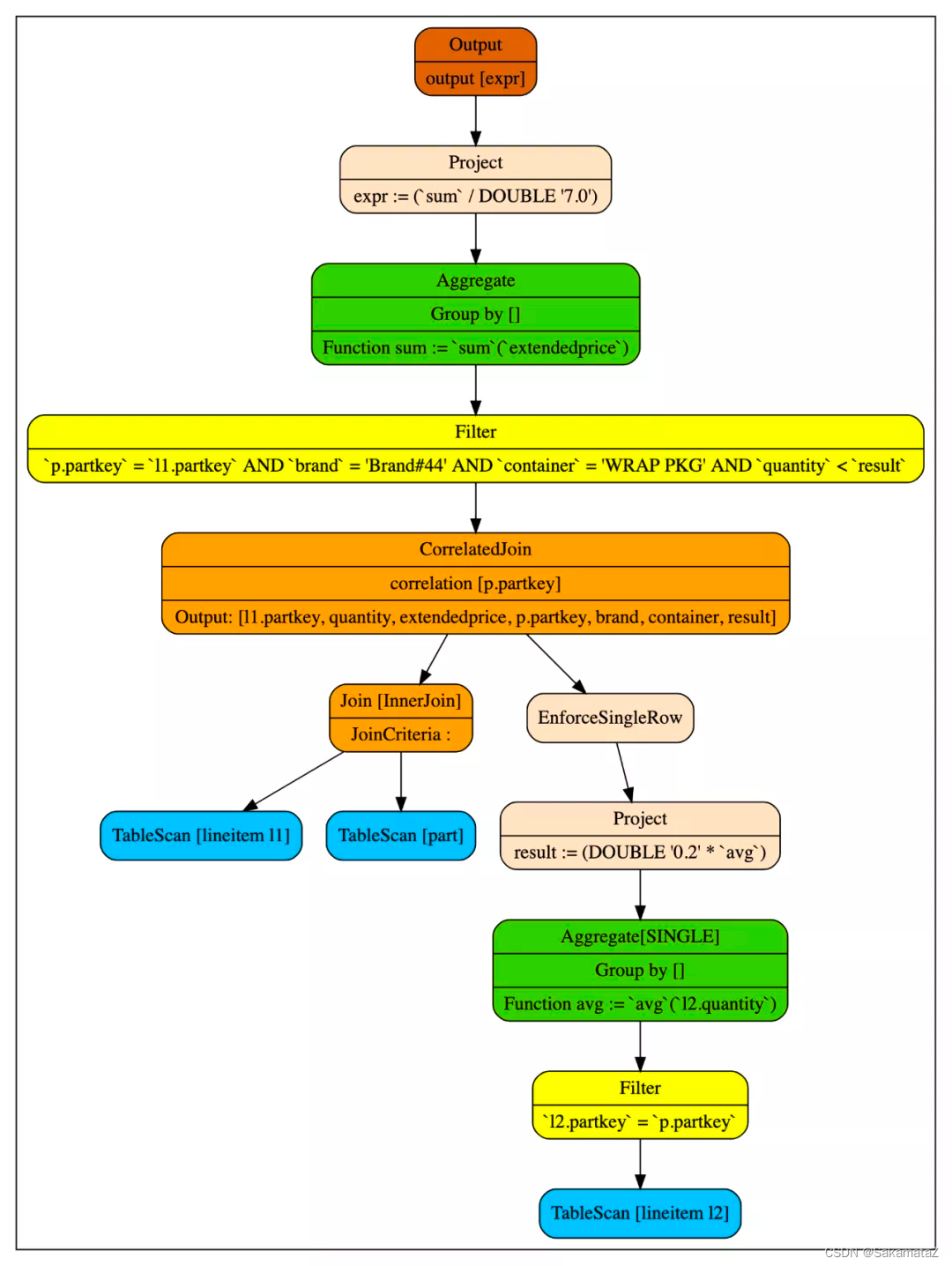
CorrelatedJoin这个算子打破了以往对逻辑树自上而下的执行模式。普通的逻辑树都是从叶子节点往根结点执行的，但是CorreltedJoin的右子树会被带入左子树的行的值反复的执行。

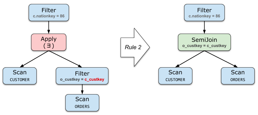
基本消除规则

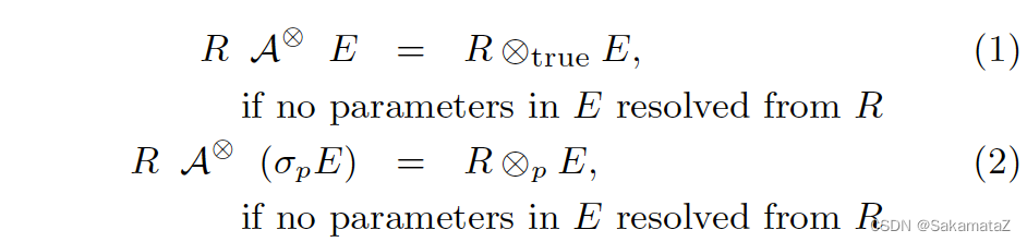
如果 Apply 的右边不包含来自左边的参数(或者只包含filter参数)，那它就和直接 Join 是等价的

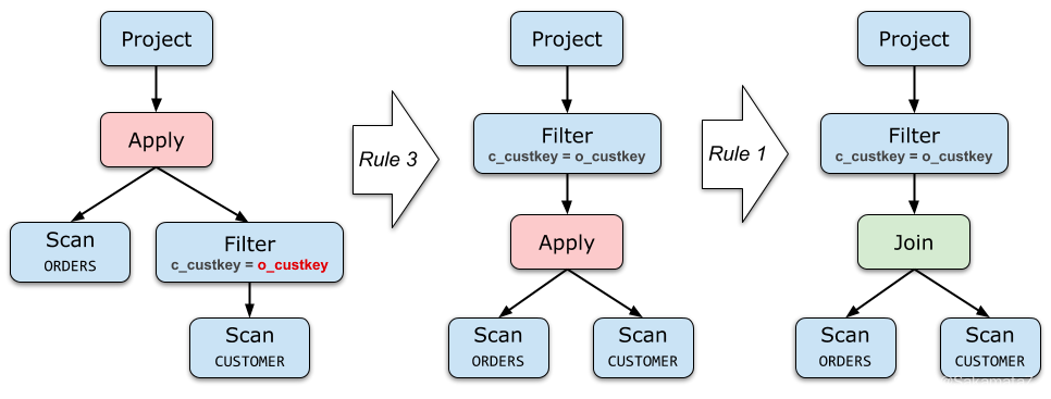
project和filter去关联化

尽可能把 Apply 往下推、把 Apply 下面的算子向上提。

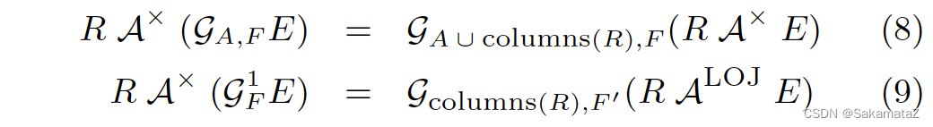
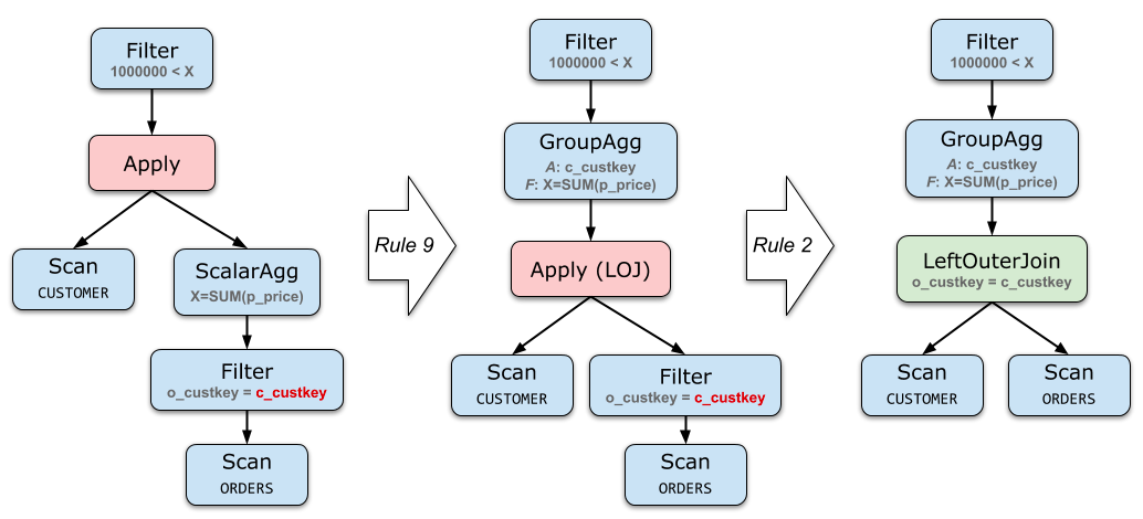
Aggregate的去关联化

SELECT c_custkey
FROM CUSTOMER
WHERE 1000000 < (
    SELECT SUM(o_totalprice)
    FROM ORDERS
    WHERE o_custkey = c_custkey
)
// 等价于
select sum(p_price) > 1000000 from CUSTOMER.o_custkey left join ORDERS.c_custkey 
on CUSTOMER.o_custkey = ORDERS.c_custkey group by ORDERS.c_custkey

集合运算的去关联化

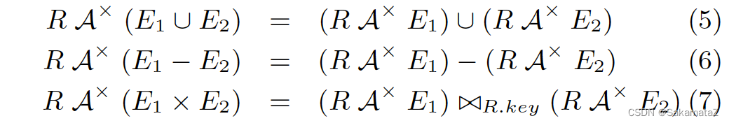
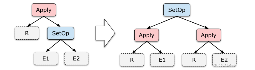
这一组规则很少能派上用场。在 TPC-H 的 Schema 下甚至很难写出一个带有 Union All 的、有意义的子查询。