Canny 边缘检测方法
Canny算子是John F.Canny 大佬在1986年在其发表的论文 《Canny J. A computational approach to edge detection [J]. IEEE Transactions on Pattern Analysis and Machine Intelligence, 1986 (6): 679-698.》提出来的。
检测目标:
- 低错误率。所有边缘都应该被找到,并且应该没有伪响应。也就是检测到的边缘必须尽可能时真实的边缘。
- 边缘点应被很好地定位。已定位边缘必须尽可能接近真实边缘。也就是由检测器标记为边缘的点和真实边缘的中心之间的距离应该最小。
- 单一的边缘点响应。这意味着在仅存一个单一边缘点的位置,检测器不应指出多个边缘像素。
Canny算法步骤
①高斯模糊 - GaussianBlur
②灰度转换 - cvtColor
③计算梯度 – Sobel/Scharr
④非最大信号抑制
⑤高低阈值输出二值图像——高低阈值比值为2:1或3:1最佳
1.灰度转换
点击图像处理之图像灰度化查看
2.高斯模糊
点击图像处理之高斯滤波查看
3.计算梯度
点击图像处理之梯度及边缘检测算子查看
4.非极大抑制
非极大值抑制是进行边缘检测的一个重要步骤,通俗意义上是指寻找像素点局部最大值。沿着梯度方向,比较它前面和后面的梯度值,如果它不是局部最大值,则去除。
在John Canny提出的Canny算子的论文中,非最大值抑制就只是在
0
∘
、
9
0
∘
、
4
5
∘
、
13
5
∘
0^\circ、90^\circ、45^\circ、135^\circ
0∘、90∘、45∘、135∘四个梯度方向上进行的,每个像素点梯度方向按照相近程度用这四个方向来代替。这四种情况也代表着四种不同的梯度,即
G
y
>
G
x
G_y>G_x
Gy>Gx,且两者同号。
G
y
>
G
x
G_y>G_x
Gy>Gx,且两者异号。
G
y
<
G
x
G_y<G_x
Gy<Gx,且两者同号。
G
y
<
G
x
G_y<G_x
Gy<Gx,且两者异号。
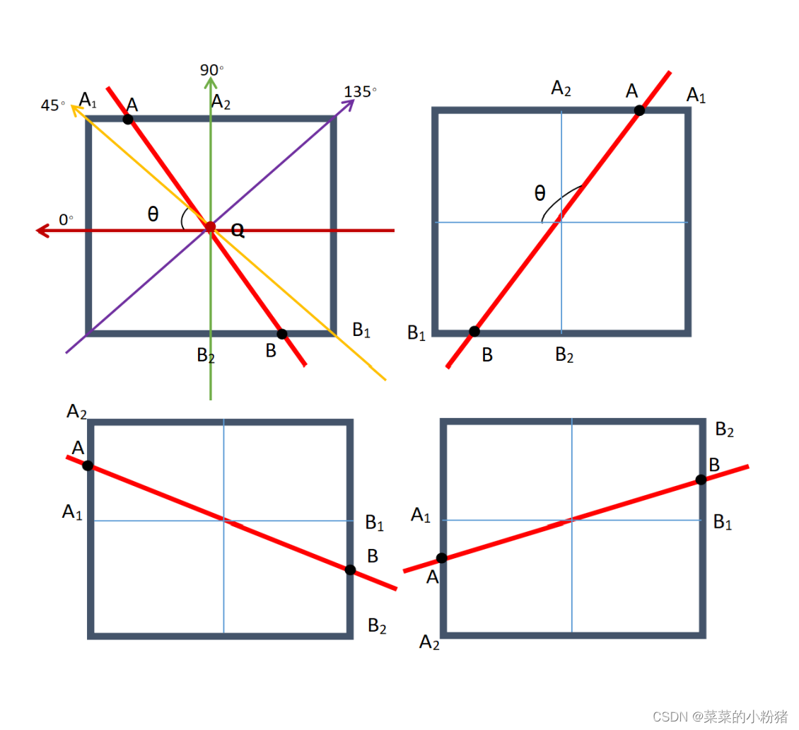
如上图所示,根据X方向和Y方向梯度的大小可以判断A点是靠近X轴还是Y轴,通过A1和A2的像素值则可计算A点的亚像素值,B点同理,不再赘述。上面两图为靠近Y轴的梯度大,下面两图为靠近X轴的像素大。
由于A、B两点的位置是通过梯度来确定的,那么A、B两点的梯度值也可以根据Q点的梯度计算,因此假设Q点在四个方向上的梯度分别为
G
1
G_1
G1、
G
2
G_2
G2、
G
3
G_3
G3、
G
4
G_4
G4。
当
G
y
>
G
x
G_y>G_x
Gy>Gx时,
w
=
G
x
G
y
,
G
1
=
(
i
−
1
,
j
)
,
G
2
=
(
i
+
1
,
j
)
w=\frac{G_x}{G_y},G_1=(i-1,j),G_2=(i+1,j)
w=GyGx,G1=(i−1,j),G2=(i+1,j)
两者同号时:
G
3
=
(
i
−
1
,
j
−
1
)
,
G
4
=
(
i
+
1
,
j
+
1
)
G_3=(i-1,j-1),G_4=(i+1,j+1)
G3=(i−1,j−1),G4=(i+1,j+1)
两者异号时:
G
3
=
(
i
−
1
,
j
+
1
)
,
G
4
=
(
i
+
1
,
j
−
1
)
G_3=(i-1,j+1),G_4=(i+1,j-1)
G3=(i−1,j+1),G4=(i+1,j−1)
当
G
y
<
G
x
G_y<G_x
Gy<Gx时,
w
=
G
y
G
x
,
G
1
=
(
i
,
j
−
1
)
,
G
2
=
(
i
,
j
+
1
)
w=\frac{G_y}{G_x},G_1=(i,j-1),G_2=(i,j+1)
w=GxGy,G1=(i,j−1),G2=(i,j+1)
两者同号时:
G
3
=
(
i
+
1
,
j
−
1
)
,
G
4
=
(
i
+
1
,
j
−
1
)
G_3=(i+1,j-1),G_4=(i+1,j-1)
G3=(i+1,j−1),G4=(i+1,j−1)
两者异号时:
G
3
=
(
i
−
1
,
j
−
1
)
,
G
4
=
(
i
+
1
,
j
+
1
)
G_3=(i-1,j-1),G_4=(i+1,j+1)
G3=(i−1,j−1),G4=(i+1,j+1)
如此便可以计算出两个相邻亚像素点的梯度值
g
A
=
w
∗
G
1
+
(
1
−
w
)
∗
G
3
g
B
=
w
∗
G
2
+
(
1
−
w
)
∗
G
4
g_A=w*G_1+(1-w)*G_3\\ g_B=w*G_2+(1-w)*G_4
gA=w∗G1+(1−w)∗G3gB=w∗G2+(1−w)∗G4
比较三者的像素值,如果Q点像素值大于其余两者,则保留Q点作为边缘上的点,否则认为Q点为冗余点。
python代码:
ef NMS(gradients, direction):
    """ Non-maxima suppression

    Args:
        gradients: the gradients of each pixel
        direction: the direction of the gradients of each pixel

    Returns:
        the output image
    """
    W, H = gradients.shape
    nms = np.copy(gradients[1:-1, 1:-1])

    for i in range(1, W - 1):
        for j in range(1, H - 1):
            theta = direction[i, j]
            weight = np.tan(theta)
            if theta > np.pi / 4:
                d1 = [0, 1]
                d2 = [1, 1]
                weight = 1 / weight
            elif theta >= 0:
                d1 = [1, 0]
                d2 = [1, 1]
            elif theta >= - np.pi / 4:
                d1 = [1, 0]
                d2 = [1, -1]
                weight *= -1
            else:
                d1 = [0, -1]
                d2 = [1, -1]
                weight = -1 / weight

            g1 = gradients[i + d1[0], j + d1[1]]
            g2 = gradients[i + d2[0], j + d2[1]]
            g3 = gradients[i - d1[0], j - d1[1]]
            g4 = gradients[i - d2[0], j - d2[1]]

            grade_count1 = g1 * weight + g2 * (1 - weight)
            grade_count2 = g3 * weight + g4 * (1 - weight)

            if grade_count1 > gradients[i, j] or grade_count2 > gradients[i, j]:
                nms[i - 1, j - 1] = 0

    return nms
5.双阈值跟踪边界
设置两个阈值,minVal和maxVal。梯度大于maxVal的任何边缘是真边缘,而minVal以下的边缘是非边缘。位于这两个阈值之间的边缘会基于其连通性而分类为边缘或非边缘,如果它们连接到“可靠边缘”像素,则它们被视为边缘的一部分;否则,不是边缘。
代码如下:
def double_threshold(nms, threshold1, threshold2):
    """ Double Threshold
    Use two thresholds to compute the edge.

    Args:
        nms: the input image
        threshold1: the low threshold
        threshold2: the high threshold

    Returns:
        The binary image.
    """

    visited = np.zeros_like(nms)
    output_image = nms.copy()
    W, H = output_image.shape

    def dfs(i, j):
        if i >= W or i < 0 or j >= H or j < 0 or visited[i, j] == 1:
            return
        visited[i, j] = 1
        if output_image[i, j] > threshold1:
            output_image[i, j] = 255
            dfs(i-1, j-1)
            dfs(i-1, j)
            dfs(i-1, j+1)
            dfs(i, j-1)
            dfs(i, j+1)
            dfs(i+1, j-1)
            dfs(i+1, j)
            dfs(i+1, j+1)
        else:
            output_image[i, j] = 0


    for w in range(W):
        for h in range(H):
            if visited[w, h] == 1:
                continue
            if output_image[w, h] >= threshold2:
                dfs(w, h)
            elif output_image[w, h] <= threshold1:
                output_image[w, h] = 0
                visited[w, h] = 1

    for w in range(W):
        for h in range(H):
            if visited[w, h] == 0:
                output_image[w, h] = 0
    return output_image
整体代码如下:
# -*- coding: utf-8 -*-
import numpy as np
import cv2
import imgShow as iS

def smooth(image, sigma = 1.4, length = 5):
    """ Smooth the image
    Compute a gaussian filter with sigma = sigma and kernal_length = length.
    Each element in the kernal can be computed as below:
        G[i, j] = (1/(2*pi*sigma**2))*exp(-((i-k-1)**2 + (j-k-1)**2)/2*sigma**2)
    Then, use the gaussian filter to smooth the input image.

    Args:
        image: array of grey image
        sigma: the sigma of gaussian filter, default to be 1.4
        length: the kernal length, default to be 5

    Returns:
        the smoothed image
    """
    # Compute gaussian filter
    k = length // 2
    gaussian = np.zeros([length, length])
    for i in range(length):
        for j in range(length):
            gaussian[i, j] = np.exp(-((i-k) ** 2 + (j-k) ** 2) / (2 * sigma ** 2))
    gaussian /= 2 * np.pi * sigma ** 2
    # Batch Normalization
    gaussian = gaussian / np.sum(gaussian)

    # Use Gaussian Filter
    W, H = image.shape
    new_image = np.zeros([W - k * 2, H - k * 2])

    for i in range(W - 2 * k):
        for j in range(H - 2 * k):
            new_image[i, j] = np.sum(image[i:i+length, j:j+length] * gaussian)

    new_image = np.uint8(new_image)

    return new_image


def get_gradient_and_direction(image):
    """ Compute gradients and its direction
    Use Sobel filter to compute gradients and direction.
         -1 0 1        -1 -2 -1
    Gx = -2 0 2   Gy =  0  0  0
         -1 0 1         1  2  1

    Args:
        image: array of grey image

    Returns:
        gradients: the gradients of each pixel
        direction: the direction of the gradients of each pixel
    """
    Gx = np.array([[-1, 0, 1], [-2, 0, 2], [-1, 0, 1]])
    Gy = np.array([[-1, -2, -1], [0, 0, 0], [1, 2, 1]])

    W, H = image.shape
    gradients = np.zeros([W - 2, H - 2])
    direction = np.zeros([W - 2, H - 2])

    for i in range(W - 2):
        for j in range(H - 2):
            dx = np.sum(image[i:i+3, j:j+3] * Gx)
            dy = np.sum(image[i:i+3, j:j+3] * Gy)
            gradients[i, j] = np.sqrt(dx ** 2 + dy ** 2)
            if dx == 0:
                direction[i, j] = np.pi / 2
            else:
                direction[i, j] = np.arctan(dy / dx)

    gradients = np.uint8(gradients)

    return gradients, direction


def NMS(gradients, direction):
    """ Non-maxima suppression

    Args:
        gradients: the gradients of each pixel
        direction: the direction of the gradients of each pixel

    Returns:
        the output image
    """
    W, H = gradients.shape
    nms = np.copy(gradients[1:-1, 1:-1])

    for i in range(1, W - 1):
        for j in range(1, H - 1):
            theta = direction[i, j]
            weight = np.tan(theta)
            if theta > np.pi / 4:
                d1 = [0, 1]
                d2 = [1, 1]
                weight = 1 / weight
            elif theta >= 0:
                d1 = [1, 0]
                d2 = [1, 1]
            elif theta >= - np.pi / 4:
                d1 = [1, 0]
                d2 = [1, -1]
                weight *= -1
            else:
                d1 = [0, -1]
                d2 = [1, -1]
                weight = -1 / weight

            g1 = gradients[i + d1[0], j + d1[1]]
            g2 = gradients[i + d2[0], j + d2[1]]
            g3 = gradients[i - d1[0], j - d1[1]]
            g4 = gradients[i - d2[0], j - d2[1]]

            grade_count1 = g1 * weight + g2 * (1 - weight)
            grade_count2 = g3 * weight + g4 * (1 - weight)

            if grade_count1 > gradients[i, j] or grade_count2 > gradients[i, j]:
                nms[i - 1, j - 1] = 0

    return nms


def double_threshold(nms, threshold1, threshold2):
    """ Double Threshold
    Use two thresholds to compute the edge.

    Args:
        nms: the input image
        threshold1: the low threshold
        threshold2: the high threshold

    Returns:
        The binary image.
    """

    visited = np.zeros_like(nms)
    output_image = nms.copy()
    W, H = output_image.shape

    def dfs(i, j):
        if i >= W or i < 0 or j >= H or j < 0 or visited[i, j] == 1:
            return
        visited[i, j] = 1
        if output_image[i, j] > threshold1:
            output_image[i, j] = 255
            dfs(i-1, j-1)
            dfs(i-1, j)
            dfs(i-1, j+1)
            dfs(i, j-1)
            dfs(i, j+1)
            dfs(i+1, j-1)
            dfs(i+1, j)
            dfs(i+1, j+1)
        else:
            output_image[i, j] = 0


    for w in range(W):
        for h in range(H):
            if visited[w, h] == 1:
                continue
            if output_image[w, h] >= threshold2:
                dfs(w, h)
            elif output_image[w, h] <= threshold1:
                output_image[w, h] = 0
                visited[w, h] = 1

    for w in range(W):
        for h in range(H):
            if visited[w, h] == 0:
                output_image[w, h] = 0

    return output_image


if __name__ == "__main__":
    # code to read image
    img=cv2.imread('./originImg/Lena.tif')
    img = cv2.cvtColor(img, cv2.COLOR_BGR2GRAY)
    smoothed_image = smooth(img)
    gradients, direction = get_gradient_and_direction(smoothed_image)
    nms = NMS(gradients, direction)
    output_image = double_threshold(nms, 40, 100)
    imageList = []
    origin_img = [img, 'origin_img']
    imageList.append(origin_img)
    # smoothed= [smoothed_image, ' smoothed_image']
    # imageList.append(smoothed)
    gradient = [gradients, 'gradients']
    imageList.append(gradient)
    nms = [nms, 'nms']
    imageList.append(nms)
    output_images = [output_image, 'output_image']
    imageList.append(output_images)
    iS.showMultipleimages(imageList, 25, 25, './ProcessedImg/canny.jpg')
检测结果: