1.基础

左偏态和右偏态指大量样本在峰顶的左边还是右边

平均值远小于中位数为左偏态，差不多为对称

西方的自然数“natural number”就是正整数,是不包括0的.

whole number为大于等于0的正整数

切比雪夫定理（Chebyshev’s theorem）：适用于任何数据集，而不论数据的分布情况如何。

与平均数的距离在z个标准差之内的数值所占的比例至少为(1-1/z²)，其中z是大于1的任意实数。

至少75%的数据值与平均数的距离在z=2个标准差之内；

至少89%的数据值与平均数的距离在z=3个标准差之内；

至少94%的数据值与平均数的距离在z=4个标准差之内；

At least none of the measurements lie in the interval μ − σ to μ + σ.

At least 3 ∕4 of the measurements lie in the interval μ − 2σ to μ + 2σ.

At least 8 ∕ 9 of the measurements lie in the interval μ − 3σ to μ + 3σ.

经验法则（Empirical Rule）：需要数据符合正态分布。

大约68%的数据值与平均数的距离在1个标准差之内；

大约95%的数据值与平均数的距离在2个标准差之内；

几乎所有的数据值与平均数的距离在3个标准差之内；

Given a distribution of measurements that is approximately mound-shaped:

The interval (μ ± σ) contains approximately 68% of the measurements.

The interval (μ ± 2σ) contains approximately 95% of the measurements.

The interval (μ ± 3σ) contains approximately 99.7% of the measurements.

The Range Approximation for sIf the range, R, is about four standard deviations, or 4s, the standard deviation can be approximated as R ≈ 4s

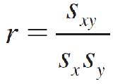
A simple measure that helps to describe this relationship is called the correlation coefficient, denoted by r, and is defined as

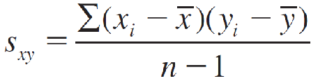
The new quantity Sxy is called the covariance between x and y and is defined as

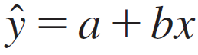
Computing Formulas for the Least-Squares Regression Line

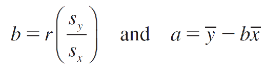
and the least-squares regression line is:

2.概率

有序：

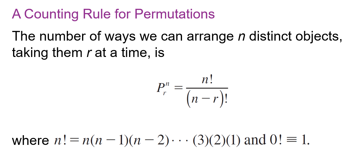
无序：

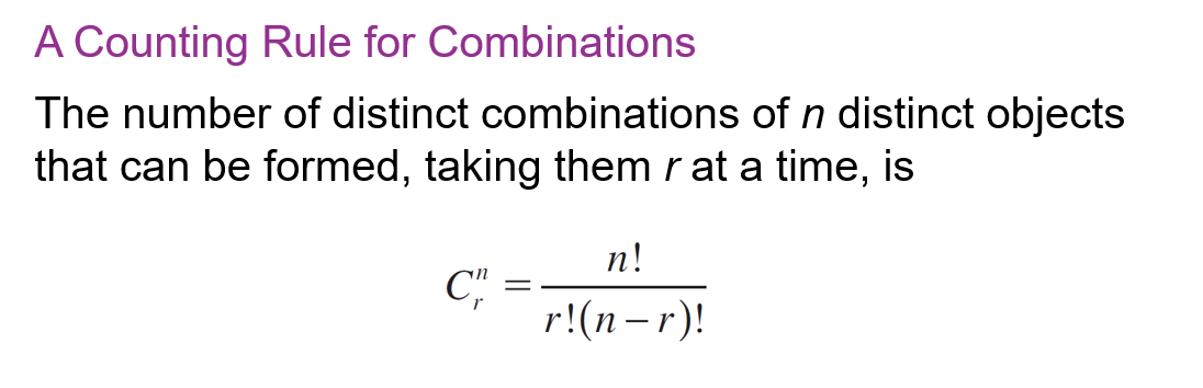
50里面选10个，有序

math.perm(50, 10)

50里面选10个，无序

math.comb(50, 10)

两个事件相互独立不一定互斥，相互独立的事件是指其中一个事件的发生不会影响另一个事件发生的概率，而互斥的事件则是指这两个事件不能同时发生。

The Addition Rule

P(A ∪ B) = P(A) + P(B) − P(A ∩ B)

When two events A and B are mutually exclusive, then P(A ∩ B) = 0 and the Addition Rule simplifies to P(A ∪ B) = P(A) + P(B)

The probability of an event A, given that the event B has occurred, is called the conditional probability of A, given that B has occurred, and written as P(A|B)

The General Multiplication RuleThe probability that both A and B occur when the experiment is performed is

P(A ∩ B) = P(A) P(B|A)

P(A ∩ B) = P(B) P(A|B)

When two events are independent—that is, if the probability of event B is the same, whether or not event A has occurred, then event A does not affect event B and P(B|A) = P(B)

The Multiplication Rule for Independent Events

If two events A and B are independent, the probability that both A and B occur is

P(A ∩ B) = P(A) P(B)

Similarly, if A, B, and C are mutually independent events (all pairs of events are independent), then the probability that A, B, and C all occur is

P(A ∩ B ∩ C) = P(A) P(B) P©

mutually exclusive events must be dependent.

When two events are mutually exclusive or disjoint,P(A ∩ B) = 0 and P(A ∪ B) = P(A) + P(B).

判断A、B两个事件是否相互独立：

Two events A and B are said to be independent if and only if either

P(A ∩ B) = P(A)P(B)

or

P(B|A) = P(B) or equivalently, P(A|B) = P(A)

Otherwise, the events are said to be dependent.

3.离散概率分布Discrete Probability Distributions

The population mean, which measures the average value of x in the population, is also called the expected value of the random variable x and is written as E(x). It is the value that you would expect to observe on average if the experiment is repeated over and over again.

Let x be a discrete random variable with probability distribution p(x). The mean or expected value of x is given as μ = E(x) = Σxp(x) summing over all the values of x.

Let x be a discrete random variable with probability distribution p(x) and mean μ. The variance of x is

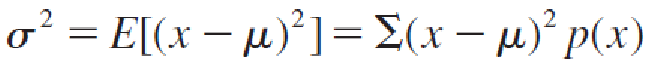
summing over all the values of x.

The Binomial Probability Distribution

Rule of Thumb

If the sample size is large relative to the population size—in particular, if n ∕ N ≥ .05—then the resulting experiment is not binomial.

The Binomial Probability Distribution

A binomial experiment consists of n identical trials with probability of success p on each trial. The probability of k successes in n trials is

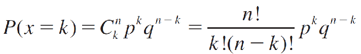
or values of k = 0, 1, 2, …, n.

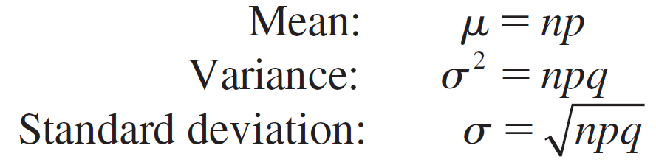
Mean and Standard Deviation for the Binomial Random VariableThe random variable x, the number of successes in n trials, has a probability distribution with this center and spread:

The Poisson Probability Distribution

Let μ be the average number of times that an event occurs in a certain period of time or space. The probability of k occurrences of this event is

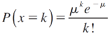
for values of k = 0, 1, 2, 3,… The mean and standard deviation of the Poisson random variable x are

Mean: μ Standard deviation: σ = √μ

How to Use Table 2 of AppendixⅠ to Calculate Poisson Probabilities

From the list, write the event as either the difference of two probabilities:

P(x ≤ a) − P(x ≤ b) for a > b 如p(4) = P(x ≤ 4) − P(x ≤ 3)

or the complement of the event:

1 − P(x ≤ a)

or just the event itself:

P(x < a) = P(x ≤ a − 1)

二项分布的泊松近似

The Poisson Approximation to the Binomial Distribution

The Poisson probability distribution provides a simple, easy-to-compute, and accurate approximation to binomial probabilities when n is large and μ = np is small, preferably with np < 7.

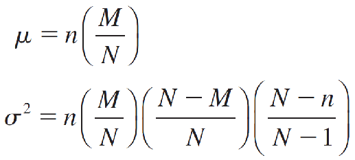
The Hypergeometric Probability Distribution

A population contains M successes and N − M failures. The probability of exactly k successes in a random sample of size n is

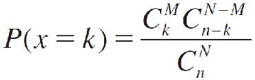
for values of k that depend on N, M, and n with

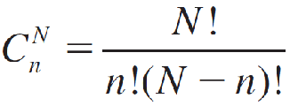
The mean and variance of a hypergeometric random variable are very similar to those of a binomial random variable with a correction for the finite population size:

4.The Normal Probability Distribution正态概率分布

Probability Distributions for Continuous Random Variables连续随机变量的概率分布

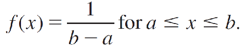
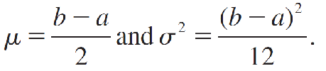
The Continuous Uniform Probability Distribution连续均匀概率分布

The continuous uniform random variable is used to model the behavior of a random variable whose values are uniformly or evenly distributed over a given interval.

If we describe this interval in general as an interval from a to b, the formula or probability density function that describes this random variable x is given by

the mean and variance of x are given by

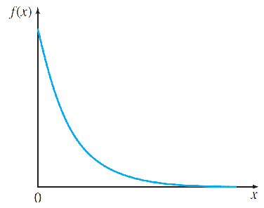
The Exponential Probability Distribution指数概率分布

The exponential random variable is used to model positive continuous random variables such as waiting times or lifetimes associated with electronic components. The probability density function is given by

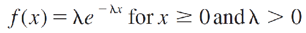
and is 0 otherwise. The parameter λ (the Greek letter “lambda”) is often referred to as the intensity and is related to the mean and variance as

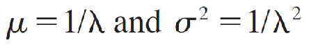
so that μ = σ.

To find areas under this curve, you can use the fact that

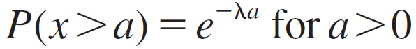
to calculate right-tailed probabilities. The left-tailed probabilities can be calculated using the complement rule as

Normal Probability Distribution

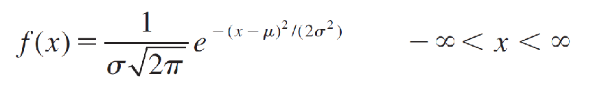
The symbols e and π are mathematical constants given approximately by 2.7183 and 3.1416, respectively; μ and σ (σ > 0) are parameters that represent the population mean and standard deviation, respectively.

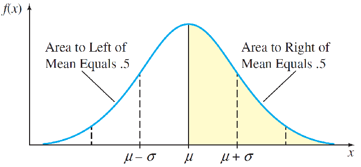
Notice the differences in shape and location. Large values of σ reduce the height of the curve and increase the spread; small values of σ increase the height of the curve and reduce the spread.

The Standard Normal Random Variable

To standardize a normal random variable x, we express its value as the number of standard deviations (σ) it lies to the left or right of its mean μ. The standardized normal random variable, z, is defined as

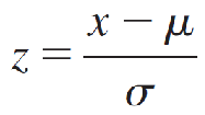
This is the familiar z-score, used to detect outliers.

标准正态分布

The probability distribution for z, shown in figure, is called the standardized normal distribution because its mean is 0 and its standard deviation is 1.

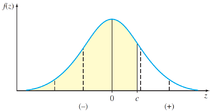
Values of z on the left side of the curve are negative, while values on the right side are positive.

The area under the standard normal curve to the left of a specified value of z—say, c—is the probability P(z ≤ c).

A common notation for a value of z having area .025 to its right is z.025 = 1.96.

The Normal Approximation to the Binomial Probability Distribution二项概率分布的正态近似

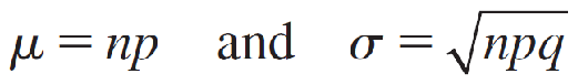
Let x be a binomial random variable with n trials and probability p of success. The probability distribution of x is approximated using a normal curve with

This approximation is adequate as long as n is large and p is not too close to 0 or 1.

The normal approximation works well when the binomial histogram is roughly symmetric. This happens when the binomial distribution is not “piled up” near 0 or n—that is, when it can spread out at least two standard deviations from its mean without exceeding its limits, 0 and n. This concept leads us to a simple rule of thumb:

Rule of Thumb

The normal approximation to the binomial probabilities will be adequate if both np > 5 and nq > 5

How to Calculate Binomial Probabilities Using the Normal Approximation

1.Find the necessary values of n and p. Calculate

2.Write the probability you need in terms of x and locate the appropriate area on the curve.

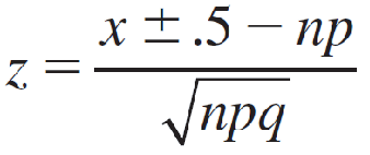
3.Correct the value of x by ±.5 to include the entire block of probability for that value. This is the continuity correction.

4.Convert the necessary x-values to z-values using

1. 当寻找 P(X > a)和P(X ≥ a) 时，从离散值 a 中减去 0.5。
2. 当寻找 P(X < a)和P(X ≤ a) 时，从离散值 a 中加上 0.5。
3. 夹在中间的时候两边分别按对应规则计算

5.Use Table 3 in Appendix I to calculate the approximate probability.

5.Sampling Distributions采样分布

Central Limit Theorem中心极限定理

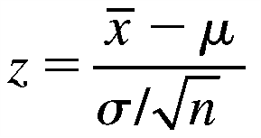
If random samples of n observations are drawn from a nonnormal population with finite mean μ and standard deviation σ, then, when n is large, the sampling distribution of the sample mean x̅ is approximately normally distributed, with mean μ and standard deviation σ/√n. The approximation becomes more accurate as n becomes large.

The Central Limit Theorem can be restated to apply to the sum of the sample measurements Σxi, which, as n becomes large, also has an approximately normal distribution with mean nμ and standard deviation σ√n

When the Sample Size Is Large Enough to Use the Central Limit Theorem：

1.If the sampled population is normal, then the sampling distribution of x̅ will also be normal, no matter what sample size you choose.

2.When the sampled population is approximately symmetric, the sampling distribution of x̅ becomes approximately normal for relatively small values of n. Remember how rapidly the discrete uniform distribution in the dice example became mound-shaped (n = 3).

3.When the sampled population is skewed, the sample size n must be larger, with n at least 30 before the sampling distribution of x̅ becomes approximately normal.

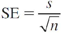
Standard Error of the Sample Mean样本均值的标准误差

The standard deviation of a statistic used as an estimator of a population parameter is also called the standard error of the estimator (abbreviated SE) because it refers to the precision of the estimator. Therefore, the standard deviation of x̅ — given by σ/√n* — is referred to as the standard error of the mean (abbreviated as SE(x̅), SEM, or sometimes just SE).

How to Calculate Probabilities for the Sample Mean x̅

If you know that the sampling distribution of x̅ is normal or approximately normal, you can describe the behavior of the sample mean x̅ by calculating the probability of observing certain values of x̅ in repeated sampling.

1. Find μ and calculate SE(x̅) = σ/√n.
2. Write down the event of interest in terms of x̅ and locate the appropriate area on the normal curve.
3. Convert the necessary values of x̅ to z-values using

4. Use Table 3 in Appendix I to calculate the probability.

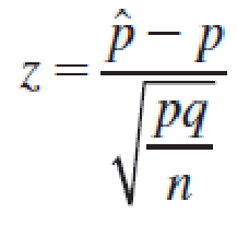
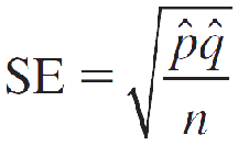
The Sampling Distribution of the Sample Proportion样本比例的抽样分布

Properties of the Sampling Distribution of the Sample Proportion, ^p

If a random sample of n observations is selected from a binomial population with parameter p, then the sampling distribution of the sample proportion

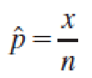
will have a mean p

and a standard deviation

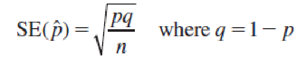
When the sample size n is large, the sampling distribution of ^p can be approximated by a normal distribution. The approximation will be adequate if np > 5 and nq > 5.

How to Calculate Probabilities for the Sample Proportion ^p

1. Find the values of n and p.

2. Check whether the normal approximation to the binomial distribution is appropriate (np > 5 and nq > 5).

3. Write down the event of interest in terms of ^p, and locate the appropriate area on the normal curve.

4. Convert the necessary values of ^p to z-values using

5. Use Table 3 in Appendix I to calculate the probability.

例题：

Random samples of size n = 90 were selected from a binomial population with p = 0.2. Use the normal distribution to approximate the following probability. (Round your answer to four decimal places.) P(0.16 ≤ ^p ≤ 0.23) = () 。

解答：

print((0.16-0.2)/math.sqrt(0.2*0.8/90))
# -0.95查表Table 3对应的Z为0.1711
print((0.23-0.2)/math.sqrt(0.2*0.8/90))
# 0.71查表Table 3对应的Z为0.7611
print(0.7611-0.1711)
# 答案为0.59

6.Large-Sample Estimation大样本估计

Point Estimation点估计

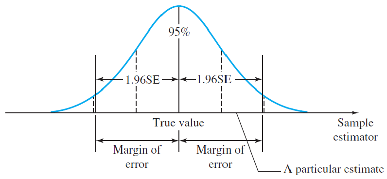
The distance between an estimate and the true value of the parameter is called the error of estimation.

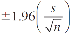
For unbiased estimators, this implies that the difference between the point estimator (the bullet) and the true value of the parameter (the bull’s-eye) will be less than 1.96 standard deviations or 1.96 standard errors (SE).

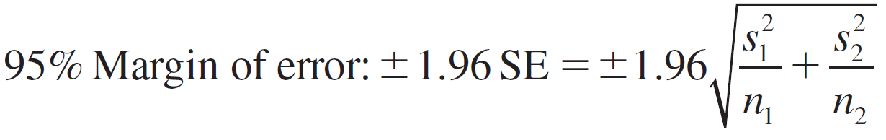
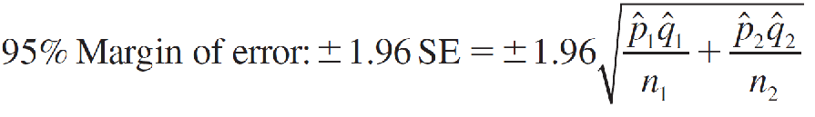
This quantity, called the 95% margin of error (or simply the “margin of error”), provides a practical upper bound for the error of estimation.

Point Estimation of a Population Parameter

1.Point estimator: a statistic calculated using sample measurements

2.95% Margin of error: 1.96×Standard error of the estimator

How to Estimate a Population Mean or Proportion

To estimate the population mean μ for a quantitative population, the point estimator x̅ is unbiased with standard error estimated as

The 95% margin of error when n ≥ 30 is estimated as

To estimate the population proportion p for a binomial population, the point estimator ^p = x/n is unbiased, with standard error estimated as

The 95% margin of error is estimated as

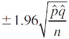
Assumptions: n ^p > 5 and n ^q > 5

例：

Suppose you are writing a questionnaire for a sample survey involving n = 484 individuals, that will generate estimates for several different binomial proportions. If you want to report a single 95% margin of error for the survey, what margin of error should you use?In order to achieve a single 95% margin of error which will work for any estimated proportion in the survey, choose a value of p which (maximize or minimize) the margin of error. Using the value p= ( ), the correct 95% margin of error, rounded to four decimal places, is().

假设您正在为涉及n = 484个个体的样本调查编写问卷，该问卷将生成几个不同的二项式比例的估计。 如果您想为调查报告单个95％边际误差，您应该使用什么边际误差？ 为了实现单个95％边际误差，该边际误差适用于调查中的任何估计比例，请选择一个p值（最大化或最小化）边际误差。 使用p =（）的值，正确的95％边际误差，四舍五入到小数点后四位，为（）。

答案：

maximize

0.5

0.0445

我们应该选择一个最大化边际误差的p值。

由于p * (1-p)在p = 0.5时取得最大值，因此我们应该选择p = 0.5来最大化边际误差。

print(1.96 * math.sqrt(0.5 * 0.5 / 484)) # 0.0445

Interval Estimation区间估计

The probability that a confidence interval will contain the estimated parameter is called the confidence coefficient.

A (1 − α)100% Large-Sample Confidence Interval

(Point estimator) ± zα ∕ 2 × (Standard error of the estimator)

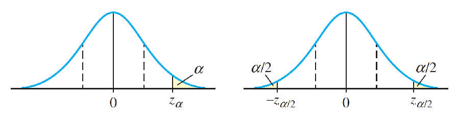
where zα ∕ 2 is the z-value with an area α ∕ 2 in the right tail of a standard normal distribution.

This formula generates two values: the lower confidence limit (LCL) and the upper confidence limit (UCL).

A (1 − α)100% Large-Sample Confidence Interval for a Population Mean

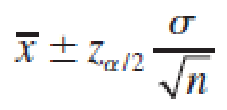
where zα ∕ 2 is the z-value corresponding to an area α ∕ 2 in the upper tail of a standard normal z distribution, and n = Sample size σ = Standard deviation of the sampled population

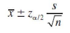
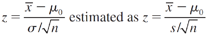
If σ is unknown, it can be approximated by the sample standard deviation s when the sample size is large (n ≥ 30) and the approximate confidence interval is

Deriving a Large-Sample Confidence Interval大样本置信区间的推导

Another way to find the large-sample confidence interval for a population mean μ is to begin with the statistic

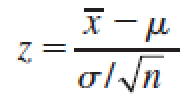
which has a standard normal distribution. If you write zα ∕ 2 as the value of z with area α ∕ 2 to its right, then you can write

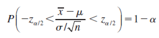
You can rewrite this inequality as

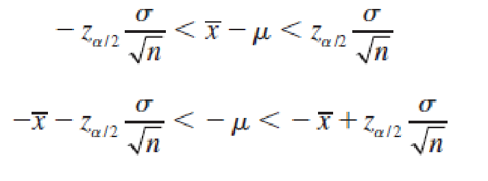
so that

Both

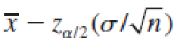
and

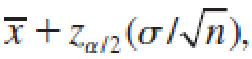
the lower and upper confidence limits, are actually random quantities that depend on the sample mean x̅.

Therefore, in repeated sampling, the random interval,

will contain the population mean μ with probability (1 − α).

Interpreting the Confidence Interval

A good confidence interval has two desirable characteristics:

1.It is as narrow as possible. The narrower the interval, the more exactly you have located the estimated parameter.

2.It has a large confidence coefficient, near 1. The larger the confidence coefficient, the more likely it is that the interval will contain the estimated parameter.

Large-Sample Confidence Interval for a Population Proportion p总体比例p的大样本置信区间

When the sample size is large, the sample proportion,

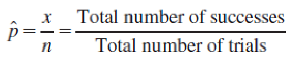
is the best point estimator for the population proportion p.

Since its sampling distribution is approximately normal, with mean p and standard error

can be used to construct a confidence interval.

A (1 − α)100% Large-Sample Confidence Interval for a Population Proportion p

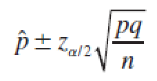
where zα ∕ 2 is the z-value corresponding to an area α ∕ 2 in the right tail of a standard normal z distribution. Since p and q are unknown, they are estimated using the best point estimators:^p and ^q.

The sample size is considered large when the normal approximation to the binomial distribution is adequate—namely, when n ^p > 5 and n ^q > 5.

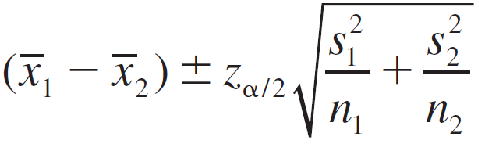
Estimating the Difference Between Two Population Means估计两个总体均值的差异

Properties of the Sampling Distribution of (x̅1 - x̅2), the Difference Between Two Sample Means

When independent random samples of n1 and n2 observations are selected from populations with means μ1 and μ2 and variances σ1² and σ2², respectively, the sampling distribution of the difference (x̅1 - x̅2) has the following properties:

1. The mean of (x̅1 - x̅2) is μ1 − μ2 and the standard error is

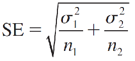
which can be estimated as

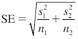
when the sample sizes are large.

2. If the sampled populations are normally distributed, then the sampling distribution of (x̅1 - x̅2) is exactly normally distributed, regardless of the sample size.
3. If the sampled populations are not normally distributed, then the sampling distribution of (x̅1 - x̅2) is approximately normally distributed when n1 and n2 are both 30 or more, due to the Central Limit Theorem.

Since (μ1 − μ2) is the mean of the sampling distribution, we know that (x̅1 - x̅2) is an unbiased estimator of (μ1 − μ2) with an approximately normal distribution when n1 and n2 are large. That is, the statistic

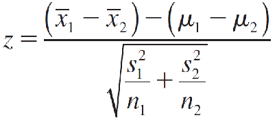
has an approximate standard normal z distribution.

Large-Sample Point Estimation of (μ1 − μ2)

Point estimator:(x̅1 - x̅2)

A (1 − α)100% Large-Sample Confidence Interval for (μ1 − μ2)

Estimating the Difference Between Two Binomial Proportions估计两个二项比例之差

Properties of the Sampling Distribution of the Difference (^p1 − ^p2) Between Two Sample Proportions

Assume that independent random samples of n1 and n2 observations have been selected from binomial populations with parameters p1 and p2, respectively.

The sampling distribution of the difference between sample proportions

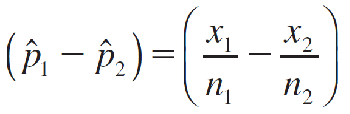
has these properties:

1. The mean of (^p1 − ^p2) is p1 − p2 and the standard error is

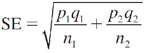
which is estimated as

2. The sampling distribution of (^p1 − ^p2) can be approximated by a normal distribution when n1 and n2 are large, due to the Central Limit Theorem.

Large-Sample Point Estimation of (p1 − p2)

Point estimator: ^p1 − ^p2

A (1 − α)100% Large-Sample Confidence Interval for (p1 − p2)

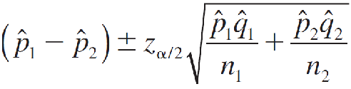
Assumption: n1 and n2 must be sufficiently large so that the sampling distribution of (^p1 − ^p2) can be approximated by a normal distribution—namely, if n1^p1, n1^q1, n2^p2, n2^q2 are all greater than 5.

One-Sided Confidence Bounds单侧置信限

A (1 − α)100% Lower Confidence Bound (LCB)

(Point estimator) − zα × (Standard error of the estimator)

A (1 − α)100% Upper Confidence Bound (UCB)

(Point estimator) + zα × (Standard error of the estimator)

7.Large-Sample Tests of Hypotheses假设的大样本检验

A Statistical Test of Hypothesis假设的统计检验

A statistical test of hypothesis consists of five parts:

1. The null hypothesis, denoted by H0
2. The alternative hypothesis, denoted by Ha
3. The test statistic and its p-value
4. The significance level and the rejection region
5. The conclusion

The two competing hypotheses are the alternative hypothesis Ha—generally the hypothesis that the researcher wishes to support—and the null hypothesis H0, a contradiction of the alternative hypothesis.

A statistical test of hypothesis begins by assuming that the null hypothesis, H0, is true. If the researcher wants to show support for the alternative hypothesis, Ha, he needs to show that H0 is false, using the sample data to decide whether the evidence favors Ha rather than H0. The researcher then draws one of two conclusions:

• Reject H0 and conclude that Ha is true.
• Accept (do not reject) H0 as true.

To decide whether to reject or accept H0, we can use two pieces of information calculated from a sample, drawn from the population of interest:

• The test statistic: a single number calculated from the sample data. The test statistic is generally based on the best estimator for the parameter to be tested.
• The p-value: a probability calculated using the test statistic

The entire set of values that the test statistic may assume is divided into two sets, or regions.

One set, consisting of values that support the alternative hypothesis and lead to rejecting H0, is called the rejection region.

The other, consisting of values that support the null hypothesis, is called the acceptance region.

When the rejection region is in the left tail of the distribution, the test is called a left-tailed test.

A test with its rejection region in the right tail is called a right-tailed test.

The level of significance (significance level) α for a statistical test of hypothesis is

α = P(falsely rejecting H0) = P(rejecting H0 when it is true)

This value a represents the maximum tolerable risk of incorrectly rejecting H0. Once this significance level is fixed, the rejection region can be set to allow the researcher to reject H0 with a fixed degree of confidence in the decision.

A Large-Sample Test About a Population Mean关于总体均值的大样本检验

The sample mean x̅ is the best estimate of the actual value of μ, which is presently in question. If H0 is true and μ = μ0, then x̅ should be fairly close to μ0. But if x̅ is much larger than μ0, this would indicate that Ha might be true.

Hence, you should reject H0 in favor of a Ha if x̅ is much larger than expected.

Since the sampling distribution of the sample mean x̅ is approximately normal when n is large, the number of standard deviations that x̅ lies from μ0 can be measured using the test statistic,

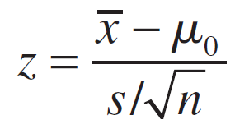
which has an approximate standard normal distribution when H0 is true and μ = μ0.

Large-Sample Statistical Test for μ

1. Null hypothesis: H0 : μ = μ0
2. Alternative hypothesis:

​ One-Tailed Test

​ Ha : μ > μ0(or, Ha : μ < μ0)

​ Two-Tailed Test

​ Ha : μ ≠ μ0

3. Test statistic:

4. Rejection region: Reject H0 when

​ One-Tailed Test

​ z > zα (or, z < −zα when thealternative hypothesis is Ha : μ < μ0)

​ Two-Tailed Test

​ z > zα/2 or z > −zα/2

Assumptions: The n observations in the sample are randomly selected from the population and n is large—say, n ≥ 30.

Calculating the p-Value

The p-value or observed significance level of a statistical test is the smallest value of α for which H0 can be rejected. It is the actual risk of committing a Type I error, if H0 is rejected based on the observed value of the test statistic. The p-value measures the strength of the evidence against H0.

A small p-value indicates that the observed value of the test statistic lies far away from the hypothesized value of μ. This presents strong evidence that H0 is false and should be rejected.

Large p-values indicate that the observed test statistic is not far from the hypothesized mean and does not support rejection of H0.

If the p-value is less than or equal to a preassigned significance level α, then the null hypothesis can be rejected, and you can report that the results are statistically significant at level α.

Use the following “sliding scale” to classify the results.

• If the p-value is less than .01, H0 is rejected. The results are highly significant.
• If the p-value is between .01 and .05, H0 is rejected. The results are statistically significant.
• If the p-value is between .05 and .10, H0 is usually not rejected. The results are only tending toward statistical significance.
• If the p-value is greater than .10, H0 is not rejected. The results are not statistically significant.

Two Types of Errors

1. The researcher might reject H0 when it is really true.
2. The researcher might accept H0 when it is really false.

For a statistical test, these two types of errors are defined as Type Ⅰ and Type Ⅱ errors, shown in Table 9.1(b).

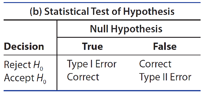
A Type Ⅰ error for a statistical test happens if you reject the null hypothesis when it is true. The probability of making a Type Ⅰ error is denoted by the symbol α.

A Type Ⅱ error for a statistical test happens if you accept the null hypothesis when it is false and some alternative hypothesis is true. The probability of making a Type Ⅱ error is denoted by the symbol β.

The Power of a Statistical Test

The power of a statistical test, given as1 − β = P(reject H0 when Ha is true)measures the ability of the test to perform as required.

A graph of (1 − β ), the probability of rejecting H0 when in fact H0 is false, as a function of the true value of the parameter of interest is called the power curve for the statistical test. Ideally, you would like a to be small and the power (1 − β ) to be large.

例：

Find the p-value for the z-test. (Round your answer to four decimal places.) a right-tailed test with observed z = 1.14

p-value =( )

对于观察到的 z = 1.14 的右尾检验，p 值等于标准正态分布中大于 1.14 的面积。

P(Z > 1.14) ≈ 0.1271

例：

Find the p-value for the z-test. (Round your answer to four decimal places.) a two-tailed test with observed variable z = −2.71

p-value =( )

对于观察到的变量 z = −2.71 的双尾检验，p 值等于标准正态分布中大于 2.71 或小于 -2.71 的面积。

P(Z > 2.71) + P(Z < -2.71) ≈ 0.0067