来源：《斯坦福数据挖掘教程·第三版》对应的公开英文书和PPT

Chapter 7 Clustering

The requirements for a function on pairs of points to be a distance measure are that:

1. Distances are always nonnegative, and only the distance between a point and itself is 0.
2. Distance is symmetric; it doesn’t matter in which order you consider the points when computing their distance.
3. Distance measures obey the triangle inequality; the distance from $x$ to $y$ to $z$ is never less than the distance going from $x$ to $z$ directly.

We can divide (cluster!) clustering algorithms into two groups that follow two fundamentally different strategies.

1. Hierarchical or agglomerative algorithms start with each point in its own cluster. Clusters are combined based on their “closeness,” using one of many possible definitions of “close.” Combination stops when further combination leads to clusters that are undesirable for one of several reasons. For example, we may stop when we have a predetermined number of
   clusters, or we may use a measure of compactness for clusters, and refuse to construct a cluster by combining two smaller clusters if the resulting cluster has points that are spread out over too large a region.
2. The other class of algorithms involve point assignment. Points are considered in some order, and each one is assigned to the cluster into which it best fits. This process is normally preceded by a short phase in which initial clusters are estimated. Variations allow occasional combining or splitting of clusters, or may allow points to be unassigned if they are outliers (points too far from any of the current clusters).

Algorithms for clustering can also be distinguished by:
(a) Whether the algorithm assumes a Euclidean space, or whether the algorithm works for an arbitrary distance measure. We shall see that a key distinction is that in a Euclidean space it is possible to summarize a collection of points by their centroid – the average of the points. In a
non-Euclidean space, there is no notion of a centroid, and we are forced to develop another way to summarize clusters.
(b) Whether the algorithm assumes that the data is small enough to fit in main memory, or whether data must reside in secondary memory, primarily. Algorithms for large amounts of data often must take shortcuts, since it is infeasible to look at all pairs of points, for example. It is also necessary to summarize clusters in main memory, since we cannot hold all the points of all the clusters in main memory at the same time.

In fact, almost all points will have a distance close to the average distance.
If there are essentially no pairs of points that are close, it is hard to build clusters at all. There is little justification for grouping one pair of points and not another. Of course, the data may not be random, and there may be useful clusters, even in very high-dimensional spaces. However, the argument about random data suggests that it will be hard to find these clusters among so many pairs that are all at approximately the same distance.

Thus, for large $d$, the cosine of the angle between any two vectors is almost certain to be close to 0, which means the angle is close to 90 degrees.
An important consequence of random vectors being orthogonal is that if we have three random points A, B, and C, and we know the distance from A to B is $d_1$, while the distance from B to C is $d_2$, we can assume the distance from A to C is approximately $\sqrt{d_1^2+d_2^2}$. That rule does not hold, even approximately, if the number of dimensions is small. As an extreme case, if $d=1$, then the distance from A to C would necessarily be $d_1+d_2$ if A and C were on opposite sides of B, or $|d_1-d_2|$ if they were on the same side.

the algorithm can be described succinctly as:

WHILE it is not time to stop DO
pick the best two clusters to merge;
combine those two clusters into one cluster;
END;

To begin, we shall assume the space is Euclidean. That allows us to represent a cluster by its centroid or average of the points in the cluster. Note that in a cluster of one point, that point is the centroid, so we can initialize the clusters straightforwardly. We can then use the merging rule that the distance between any two clusters is the Euclidean distance between their centroids, and we should pick the two clusters at the shortest distance.

There are several approaches we might use to stopping the clustering process.

1. We could be told, or have a belief, about how many clusters there are in the data. For example, if we are told that the data about dogs is taken from Chihuahuas, Dachshunds, and Beagles, then we know to stop when there are three clusters left.
2. We could stop combining when at some point the best combination of existing clusters produces a cluster that is inadequate. But for an example, we could insist that any cluster have an average distance between the centroid and its points no greater than some limit. This approach is only sensible if we have a reason to believe that no cluster extends over too much of the space.
3. We could continue clustering until there is only one cluster. However, it is meaningless to return a single cluster consisting of all the points. Rather, we return the tree representing the way in which all the points were combined. This form of answer makes good sense in some applications, such as one in which the points are genomes of different species, and the distance measure reflects the difference in the genome.2 Then, the tree represents the evolution of these species, that is, the likely order in which two species branched from a common ancestor.

Efficiency of Hierarchical Clustering

The basic algorithm for hierarchical clustering is not very efficient. At each step, we must compute the distances between each pair of clusters, in order to find the best merger. The initial step takes $O(n^2)$ time, but subsequent steps take time proportional to $(n-1{)}^2,(n-2{)}^2,....$ The sum of squares up to n is $O(n^3)$, so this algorithm is cubic. Thus, it cannot be run except for fairly small numbers of points.

However, there is a somewhat more efficient implementation of which we should be aware.

1. We start, as we must, by computing the distances between all pairs of points, and this step is $O(n^2).$
2. Form the pairs and their distances into a priority queue, so we can always find the smallest distance in one step. This operation is also $O(n^2)$.
3. When we decide to merge two clusters C and D, we remove all entries in the priority queue involving one of these two clusters; that requires work $O(nlogn)$ since there are at most $2n$ deletions to be performed, and priority-queue deletion can be performed in $O(logn)$ time.
4. We then compute all the distances between the new cluster and the remaining clusters. This work is also $O(nlogn)$ , as there are at most n entries to be inserted into the priority queue, and insertion into a priority queue can also be done in $O(logn)$ time.

Since the last two steps are executed at most n times, and the first two steps are executed only once, the overall running time of this algorithm is $O(n^{2}logn)$. That is better than $O(n^3)$, but it still puts a strong limit on how large n can be before it becomes infeasible to use this clustering approach.

We have seen one rule for picking the best clusters to merge: find the pair with the smallest distance between their centroids. Some other options are:

1. Take the distance between two clusters to be the minimum of the distances between any two points, one chosen from each cluster.
2. Take the distance between two clusters to be the average distance of all pairs of points, one from each cluster.
3. The radius of a cluster is the maximum distance between all the points and the centroid. Combine the two clusters whose resulting cluster has the lowest radius. A slight modification is to combine the clusters whose result has the lowest average distance between a point and the centroid. Another modification is to use the sum of the squares of the distances between the points and the centroid. In some algorithms, we shall find these variant definitions of “radius” referred to as “the radius.”
4. The diameter of a cluster is the maximum distance between any two points of the cluster. Note that the radius and diameter of a cluster are not related directly, as they are in a circle, but there is a tendency for them to be proportional. We may choose to merge those clusters whose resulting cluster has the smallest diameter. Variants of this rule, analogous to the rule for radius, are possible.

We also have options in determining when to stop the merging process. We already mentioned “stop when we have k clusters” for some predetermined k. Here are some other options.

1. Stop if the diameter of the cluster that results from the best merger exceeds a threshold. We can also base this rule on the radius, or on any of the variants of the radius mentioned above.
2. Stop if the density of the cluster that results from the best merger is below some threshold. The density can be defined in many different ways. Roughly, it should be the number of cluster points per unit volume of the cluster. That ratio can be estimated by the number of points divided by some power of the diameter or radius of the cluster. The correct power could be the number of dimensions of the space. Sometimes, 1 or 2 is chosen as the power, regardless of the number of dimensions.
3. Stop when there is evidence that the next pair of clusters to be combined yields a bad cluster. For example, we could track the average diameter of all the current clusters. As long as we are combining points that truly belong in a cluster, this average will rise gradually. However, if we combine two clusters that really don’t deserve to be combined, then the average diameter will take a sudden jump.

Given that we cannot combine points in a cluster when the space is non-Euclidean, our only choice is to pick one of the points of the cluster itself to represent the cluster. Ideally, this point is close to all the points of the cluster, so it in some sense lies in the “center.” We call the representative point the clustroid. We can select the clustroid in various ways, each designed to, in some sense, minimize the distances between the clustroid and the other points in the cluster. Common choices include selecting as the clustroid the point that minimizes:

1. The sum of the distances to the other points in the cluster.
2. The maximum distance to another point in the cluster.
3. The sum of the squares of the distances to the other points in the cluster.

Initially choose k points that are likely to be in different clusters;
Make these points the centroids of their clusters;
FOR each remaining point p DO
find the centroid to which p is closest;
Add p to the cluster of that centroid;
Adjust the centroid of that cluster to account for p;
END;

We want to pick points that have a good chance of lying in different clusters. There are two approaches.

1. Pick points that are as far away from one another as possible.
2. Cluster a sample of the data, perhaps hierarchically, so there are k clusters. Pick a point from each cluster, perhaps that point closest to the centroid of the cluster.

The second approach requires little elaboration. For the first approach, there are variations. One good choice is:

Pick the first point at random;
WHILE there are fewer than k points DO
Add the point whose minimum distance from the selected
points is as large as possible;
END;

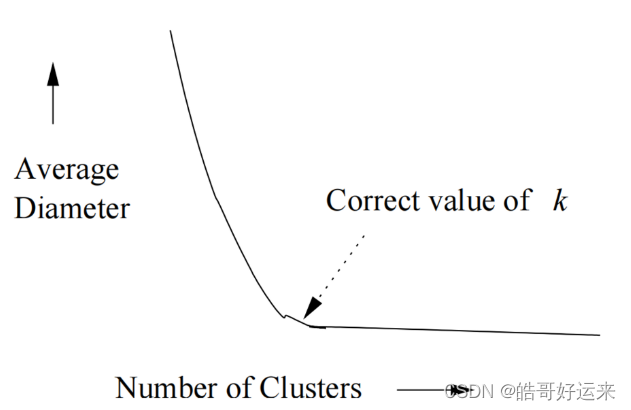
Average diameter or another measure of diffuseness rises quickly as soon as the number of clusters falls below the true number present in the data。

If we have no idea what the correct value of $k$ is, we can find a good value in a number of clustering operations that grows only logarithmically with the true number. Begin by running the k-means algorithm for $k=1,2,4,8,....$ Eventually, you will find two values $v$ and $2v$ between which there is very little decrease in the average diameter, or whatever measure of cluster cohesion you are using. We may conclude that the value of k that is justified by the data lies between $\frac{v}{2}$ and $v$. If you use a binary search in that range, you can find the best value for $k$ in another $lo{g}_{2}v$ clustering operations, for a total of $2lo{g}_{2}v$ clusterings. Since the true value of $k$ is at least $\frac{v}{2}$, we have used a number of clusterings that is logarithmic in $k$.

The Algorithm of Bradley, Fayyad, and Reina(BFR)

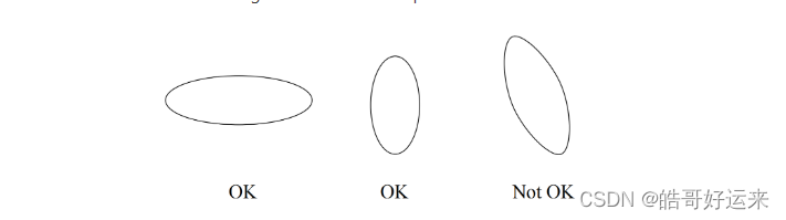
The Algorithm of Bradley, Fayyad, and Reina(BFR) makes a very strong assumption about the shape of clusters: they must be normally distributed about a centroid. The mean and standard deviation for a cluster may differ for different dimensions, but the dimensions must be independent. For instance, in two dimensions a cluster may be cigar-shaped, but the cigar must not be rotated off of the axes. Figure 7.10 makes the point.

The BFR Algorithm begins by selecting k points. Then, the points of the data file are read in chunks. These might be chunks from a distributed file system or a conventional file might be partitioned into chunks of the appropriate size. Each chunk must consist of few enough points that they can be processed in main memory. Also stored in main memory are summaries of the k clusters and some other data, so the entire memory is not available to store a chunk. The main-memory data other than the chunk from the input consists of three types of objects:

1. The Discard Set: These are simple summaries of the clusters themselves. We shall address the form of cluster summarization shortly. Note that the cluster summaries are not “discarded”; they are in fact essential. However, the points that the summary represents are discarded and have no representation in main memory other than through this summary.
2. The Compressed Set: These are summaries, similar to the cluster summaries, but for sets of points that have been found close to one another, but not close to any cluster. The points represented by the compressed set are also discarded, in the sense that they do not appear explicitly in main memory. We call the represented sets of points miniclusters.
3. The Retained Set: Certain points can neither be assigned to a cluster nor are they sufficiently close to any other points that we can represent them by a compressed set. These points are held in main memory exactly as they appear in the input file.

The discard and compressed sets are represented by $2d+1$ values, if the data is d-dimensional. These numbers are:

(a) The number of points represented, N.

(b) The sum of the components of all the points in each dimension. This data is a vector SUM of length d, and the component in the ith dimension is $SU{M}_i$.

© The sum of the squares of the components of all the points in each dimension. This data is a vector SUMSQ of length d, and its component in the ith dimension is $SUMS{Q}_i$.

Our real goal is to represent a set of points by their count, their centroid and the standard deviation in each dimension. However, these $2d+1$ values give us those statistics. N is the count. The centroid’s coordinate in the ith dimension is the $SU{M}_i/N$, that is the sum in that dimension divided by the number of points. The variance in the ith dimension is $SUMS{Q}_i/N-(SUMi/N{)}^2$. We can compute the standard deviation in each dimension, since it is the square root of the variance.

We shall now outline what happens when we process a chunk of points.

1. First, all points that are sufficiently close to the centroid of a cluster are added to that cluster. It is simple to add the information about the point to the N, SUM, and SUMSQ that represent the cluster. We then discard the point. The question of what “sufficiently close” means will be addressed shortly.
2. For the points that are not sufficiently close to any centroid, we cluster them, along with the points in the retained set. Any main-memory clustering algorithm can be used. We must use some criterion for deciding when it is reasonable to combine two points into a cluster or two clusters into one. Clusters of more than one point are summarized and added to the compressed set. Singleton clusters become the retained set of points.
3. We now have miniclusters derived from our attempt to cluster new points and the old retained set, and we have the miniclusters from the old compressed set. Although none of these miniclusters can be merged with one of the k clusters, they might merge with one another. Note that the form of representation for compressed sets (N, SUM, and
   SUMSQ) makes it easy to compute statistics such as the variance for the combination of two miniclusters that we consider merging.
4. Points that are assigned to a cluster or a minicluster, i.e., those that are not in the retained set, are written out, with their assignment, to secondary memory.

Finally, if this is the last chunk of input data, we need to do something with the compressed and retained sets. We can treat them as outliers, and never cluster them at all. Or, we can assign each point in the retained set to the cluster of the nearest centroid. We can combine each minicluster with the cluster whose centroid is closest to the centroid of the minicluster.

An important decision that must be examined is how we decide whether a new point p is close enough to one of the k clusters that it makes sense to add p to the cluster. Two approaches have been suggested.

(a) Add p to a cluster if it not only has the centroid closest to p, but it is very unlikely that, after all the points have been processed, some other cluster centroid will be found to be nearer to p. This decision is a complex statistical calculation. It must assume that points are ordered randomly, and that we know how many points will be processed in the future. Its advantage is that if we find one centroid to be significantly closer to p than any other, we can add p to that cluster and be done with it, even if p is very far from all centroids.
(b) We can measure the probability that, if p belongs to a cluster, it would be found as far as it is from the centroid of that cluster. This calculation makes use of the fact that we believe each cluster to consist of normally distributed points with the axes of the distribution aligned with the axes of the space. It allows us to make the calculation through the Mahalanobis distance of the point.

The Mahalanobis distance is essentially the distance between a point and the centroid of a cluster, normalized by the standard deviation of the cluster in each dimension. Since the BFR Algorithm assumes the axes of the cluster align with the axes of the space, the computation of Mahalanobis distance is especially simple. Let $p=[p1,p2,...,pd]$ be a point and $c=[c1,c2,...,cd]$ the centroid of a cluster. Let ${\sigma }_i$ be the standard deviation of points in the cluster in the ith dimension. Then the Mahalanobis distance between p and c is

$$\sqrt{\sum _{i=1}^d(\frac{p_i-c_i}{{\sigma }_i}{)}^2}$$

That is, we normalize the difference between p and c in the ith dimension by dividing by the standard deviation of the cluster in that dimension. The rest of the formula combines the normalized distances in each dimension in the normal way for a Euclidean space.
To assign point p to a cluster, we compute the Mahalanobis distance between p and each of the cluster centroids. We choose that cluster whose centroid has the least Mahalanobis distance, and we add p to that cluster provided the Mahalanobis distance is less than a threshold. For instance, suppose we pick four as the threshold. If data is normally distributed, then the probability of a value as far as four standard deviations from the mean is less than one in a million. Thus, if the points in the cluster are really normally distributed, then the probability that we will fail to include a point that truly belongs is less than $10^{-6}$. And such a point is likely to be assigned to that cluster eventually anyway, as long as it does not wind up closer to some other centroid as centroids migrate in response to points added to their cluster.

The CURE Algorithm

We now turn to another large-scale-clustering algorithm in the point-assignment class. This algorithm, called CURE (Clustering Using REpresentatives), assumes a Euclidean space. However, it does not assume anything about the shape of clusters; they need not be normally distributed, and can even have strange bends, S-shapes, or even rings. Instead of representing clusters by their centroid, it uses a collection of representative points, as the name implies.

We begin the CURE algorithm by:

1. Take a small sample of the data and cluster it in main memory. In principle, any clustering method could be used, but as CURE is designed to handle oddly shaped clusters, it is often advisable to use a hierarchical method in which clusters are merged when they have a close pair of points.
2. Select a small set of points from each cluster to be representative points. These points should be chosen to be as far from one another as possible.
3. Move each of the representative points a fixed fraction of the distance between its location and the centroid of its cluster. Perhaps 20% is a good fraction to choose. Note that this step requires a Euclidean space, since otherwise, there might not be any notion of a line between two points.

The next phase of CURE is to merge two clusters if they have a pair of representative points, one from each cluster, that are sufficiently close. The user may pick the distance that defines “close.” This merging step can repeat, until there are no more sufficiently close clusters.

The GRGPF algorithm

We shall next consider an algorithm that handles non-main-memory data, but does not require a Euclidean space. The algorithm, which we shall refer to as GRGPF for its authors (V. Ganti, R. Ramakrishnan, J. Gehrke, A. Powell, and J. French), takes ideas from both hierarchical and point-assignment approaches. Like CURE, it represents clusters by sample points in main memory. However, it also tries to organize the clusters hierarchically, in a tree, so a new point can be assigned to the appropriate cluster by passing it down the tree. Leaves of the tree hold summaries of some clusters, and interior nodes hold subsets of the information describing the clusters reachable through that node. An attempt is made to group clusters by their distance from one another, so the clusters at a leaf are close, and the clusters reachable from one interior node are relatively close as well.

As we assign points to clusters, the clusters can grow large. Most of the points in a cluster are stored on disk, and are not used in guiding the assignment of points, although they can be retrieved. The representation of a cluster in main memory consists of several features. Before listing these features, if p is any point in a cluster, let $ROWSUM(p)$ be the sum of the squares of the distances from p to each of the other points in the cluster. Note that, although we are not in a Euclidean space, there is some distance measure d that applies to points, or else it is not possible to cluster points at all. The following features form the representation of a cluster.

1. N, the number of points in the cluster.
2. The clustroid of the cluster, which is defined specifically to be the point in the cluster that minimizes the sum of the squares of the distances to the other points; that is, the clustroid is the point in the cluster with the smallest ROWSUM.
3. The rowsum of the clustroid of the cluster.
4. For some chosen constant k, the k points of the cluster that are closest to the clustroid, and their rowsums. These points are part of the representation in case the addition of points to the cluster causes the clustroid to change. The assumption is made that the new clustroid would be one of these k points near the old clustroid.
5. The k points of the cluster that are furthest from the clustroid and their rowsums. These points are part of the representation so that we can consider whether two clusters are close enough to merge. The assumption is made that if two clusters are close, then a pair of points distant from their respective clustroids would be close.

An interior node of the cluster tree holds a sample of the clustroids of the clusters represented by each of its subtrees, along with pointers to the roots of those subtrees. The samples are of fixed size, so the number of children that an interior node may have is independent of its level. Notice that as we go up the tree, the probability that a given cluster’s clustroid is part of the sample diminishes.
We initialize the cluster tree by taking a main-memory sample of the dataset and clustering it hierarchically. The result of this clustering is a tree T , but T is not exactly the tree used by the GRGPF Algorithm. Rather, we select from T certain of its nodes that represent clusters of approximately some desired size n. These are the initial clusters for the GRGPF Algorithm, and we place their representations at the leaf of the cluster-representing tree. We then group clusters with a common ancestor in T into interior nodes of the cluster-representing tree, so in some sense, clusters descended from one interior node are as close as possible. In some cases, rebalancing of the cluster-representing tree will be necessary. This process is similar to the reorganization of a B-tree, and we shall not examine this issue in detail.

We now read points from secondary storage and insert each one into the nearest cluster. We start at the root, and look at the samples of clustroids for each of the children of the root. Whichever child has the clustroid closest to the new point p is the node we examine next. When we reach any node in the tree, we look at the sample clustroids for its children and go next to the child with the clustroid closest to p. Note that some of the sample clustroids at a node may
have been seen at a higher level, but each level provides more detail about the clusters lying below, so we see many new sample clustroids each time we go a level down the tree.
Finally, we reach a leaf. This leaf has the cluster features for each cluster represented by that leaf, and we pick the cluster whose clustroid is closest to p. We adjust the representation of this cluster to account for the new node p. In particular, we:

1. Add 1 to N.

2. Add the square of the distance between p and each of the nodes q mentioned in the representation to ROWSUM(q). These points q include the clustroid, the k nearest points, and the k furthest points. We also estimate the rowsum of p, in case p needs to be part of the representation (e.g., it turns out to be one of the k points closest to the clustroid). Note we cannot compute ROWSUM§ exactly, without going to disk and retrieving all the points of the cluster. The estimate we use is

   $$ROWSUM(p)=ROWSUM(c)+N{d}^2(p,c)$$

   where $d(p,c)$ is the distance between p and the clustroid c. Note that N and ROWSUM© in this formula are the values of these features before they were adjusted to account for the addition of p.

We might well wonder why this estimate works. Typically a non-Euclidean space also suffers from the curse of dimensionality, in that it behaves in many ways like a high-dimensional Euclidean space. If we assume that the angle between p, c, and another point q in the cluster is a right angle, then the Pythagorean theorem tell us that

$$d^2(p,q)=d^2(p,c)+d^2(c,q)$$

If we sum over all q other than c, and then add $d^2(p,c)$ to ROWSUM§ to account for the fact that the clustroid is one of the points in the cluster, we derive $ROWSUM(p)=ROWSUM(c)+N{d}^2(p,c)$.
Now, we must see if the new point p is one of the k closest or furthest points from the clustroid, and if so, p and its rowsum become a cluster feature, replacing one of the other features – whichever is no longer one of the k closest or furthest. We also need to consider whether the rowsum for one of the k closest points q is now less than ROWSUM©. That situation could happen if p were closer to one of these points than to the current clustroid. If so, we swap the roles of c and q. Eventually, it is possible that the true clustroid will no longer be one of the original k closest points. We have no way of knowing, since we do not see the other points of the cluster in main memory. However, they are all stored on disk, and can be brought into main memory periodically for a recomputation of the cluster features.

The GRGPF Algorithm assumes that there is a limit on the radius that a cluster may have. The particular definition used for the radius is $\sqrt{ROWSUM(c)/N}$, where c is the clustroid of the cluster and N the number of points in the cluster. That is, the radius is the square root of the average square of the distance from the clustroid of the points in the cluster. If a cluster’s radius grows too large, it is split into two. The points of that cluster are brought into main memory, and divided into two clusters to minimize the rowsums. The cluster features for both clusters are computed.
As a result, the leaf of the split cluster now has one more cluster to represent. We should manage the cluster tree like a B-tree, so usually, there will be room in a leaf to add one more cluster. However, if not, then the leaf must be split into two leaves. To implement the split, we must add another pointer and more sample clustroids at the parent node. Again, there may be extra space, but if not, then this node too must be split, and we do so to minimize the squares of the distances between the sample clustroids assigned to different nodes. As in a B-tree, this splitting can ripple all the way up to the root, which can then be split if needed.

The worst thing that can happen is that the cluster-representing tree is now too large to fit in main memory. There is only one thing to do: we make it smaller by raising the limit on how large the radius of a cluster can be, and we consider merging pairs of clusters. It is normally sufficient to consider clusters that are “nearby,” in the sense that their representatives are at the same leaf or at leaves with a common parent. However, in principle, we can consider merging any two clusters $C_1$ and $C_2$ into one cluster C. To merge clusters, we assume that the clustroid of C will be one of the points that are as far as possible from the clustroid of $C_1$ or the clustroid of $C_2$. Suppose we want to compute the rowsum in C for the point p, which is one of the k points in $C_1$ that are as far as possible from the centroid of $C_1$. We use the curse-of-dimensionality argument that says all angles are approximately right angles, to justify the following formula.

In the above, we subscript N and ROWSUM by the cluster to which that feature refers. We use $c_1$ and $c_2$ for the clustroids of $C_1$ and $C_2$, respectively.

In detail, we compute the sum of the squares of the distances from p to all the nodes in the combined cluster C by beginning with $ROWSU{M}_{C_1}(p)$ to get the terms for the points in the same cluster as p. For the $N_{C_2}$ points q in $C_2$, we consider the path from p to the clustroid of $C_1$, then to the clustroid of $C_2$, and finally to q. We assume there is a right angle between the legs from p to $c_1$ and $c_1$ to $c_2$, and another right angle between the shortest path from p to
$c_2$ and the leg from $c_2$ to q. We then use the Pythagorean theorem to justify computing the square of the length of the path to each q as the sum of the squares of the three legs.
We must then finish computing the features for the merged cluster. We need to consider all the points in the merged cluster for which we know the rowsum. These are, the centroids of the two clusters, the k points closest to the clustroids for each cluster, and the k points furthest from the clustroids for each cluster, with the exception of the point that was chosen as the new clustroid.
We can compute the distances from the new clustroid for each of these $4k+1$ points. We select the k with the smallest distances as the “close” points and the k with the largest distances as the “far” points. We can then compute the rowsums for the chosen points, using the same formulas above that we used to compute the rowsums for the candidate clustroids.

Summary of Chapter 7

• Clustering: Clusters are often a useful summary of data that is in the form of points in some space. To cluster points, we need a distance measure on that space. Ideally, points in the same cluster have small distances between them, while points in different clusters have large distances between them.
• Clustering Algorithms: Clustering algorithms generally have one of two forms. Hierarchical clustering algorithms begin with all points in a cluster of their own, and nearby clusters are merged iteratively. Point-assignment clustering algorithms consider points in turn and assign them to the cluster in which they best fit.
• The Curse of Dimensionality: Points in high-dimensional Euclidean spaces, as well as points in non-Euclidean spaces often behave unintuitively. Two unexpected properties of these spaces are that random points are almost always at about the same distance, and random vectors are almost always orthogonal.
• Centroids and Clustroids: In a Euclidean space, the members of a cluster can be averaged, and this average is called the centroid. In non-Euclidean spaces, there is no guarantee that points have an “average,” so we are forced to use one of the members of the cluster as a representative or typical element of the cluster. That representative is called the clustroid.
• Choosing the Clustroid: There are many ways we can define a typical point of a cluster in a non-Euclidean space. For example, we could choose the point with the smallest sum of distances to the other points, the smallest sum of the squares of those distances, or the smallest maximum distance to any other point in the cluster.
• Radius and Diameter: Whether or not the space is Euclidean, we can define the radius of a cluster to be the maximum distance from the centroid or clustroid to any point in that cluster. We can define the diameter of the cluster to be the maximum distance between any two points in the cluster. Alternative definitions, especially of the radius, are also known, for example, average distance from the centroid to the other points.
• Hierarchical Clustering: This family of algorithms has many variations, which differ primarily in two areas. First, we may chose in various ways which two clusters to merge next. Second, we may decide when to stop the merge process in various ways.
• Picking Clusters to Merge: One strategy for deciding on the best pair of clusters to merge in a hierarchical clustering is to pick the clusters with the closest centroids or clustroids. Another approach is to pick the pair of clusters with the closest points, one from each cluster. A third approach is to use the average distance between points from the two clusters.
• Stopping the Merger Process: A hierarchical clustering can proceed until there are a fixed number of clusters left. Alternatively, we could merge until it is impossible to find a pair of clusters whose merger is sufficiently compact, e.g., the merged cluster has a radius or diameter below some threshold. Another approach involves merging as long as the resulting cluster has a sufficiently high “density,” which can be defined in various ways, but is the number of points divided by some measure of the size of the cluster, e.g., the radius.
• K-Means Algorithms: This family of algorithms is of the point-assignment type and assumes a Euclidean space. It is assumed that there are exactly k clusters for some known k. After picking k initial cluster centroids, the points are considered one at a time and assigned to the closest centroid. The centroid of a cluster can migrate during point assignment, and an optional last step is to reassign all the points, while holding the centroids fixed at their final values obtained during the first pass.
• Initializing K-Means Algorithms: One way to find k initial centroids is to pick a random point, and then choose $k-1$ additional points, each as far away as possible from the previously chosen points. An alternative is to start with a small sample of points and use a hierarchical clustering to merge them into k clusters.
• Picking K in a K-Means Algorithm: If the number of clusters is unknown, we can use a binary-search technique, trying a k-means clustering with different values of k. We search for the largest value of k for which a decrease below k clusters results in a radically higher average diameter of the clusters. This search can be carried out in a number of clustering operations that is logarithmic in the true value of k.
• The BFR Algorithm: This algorithm is a version of k-means designed to handle data that is too large to fit in main memory. It assumes clusters are normally distributed about the axes.
• Representing Clusters in BFR: Points are read from disk one chunk at a time. Clusters are represented in main memory by the count of the number of points, the vector sum of all the points, and the vector formed by summing the squares of the components of the points in each dimension. Other collection of points, too far from a cluster centroid to be included in a cluster, are represented as “miniclusters” in the same way as the k
  clusters, while still other points, which are not near any other point will be represented as themselves and called “retained” points.
• Processing Points in BFR: Most of the points in a main-memory load will be assigned to a nearby cluster and the parameters for that cluster will be adjusted to account for the new points. Unassigned points can be formed into new miniclusters, and these miniclusters can be merged with previously discovered miniclusters or retained points. After the last memory load, the miniclusters and retained points can be merged to their nearest cluster or kept as outliers.
• The CURE Algorithm: This algorithm is of the point-assignment type. It is designed for a Euclidean space, but clusters can have any shape. It handles data that is too large to fit in main memory.
• Representing Clusters in CURE: The algorithm begins by clustering a small sample of points. It then selects representative points for each cluster, by picking points in the cluster that are as far away from each other as possible. The goal is to find representative points on the fringes of the cluster. However, the representative points are then moved a fraction of the way toward the centroid of the cluster, so they lie somewhat in the interior of the cluster.
• Processing Points in CURE: After creating representative points for each cluster, the entire set of points can be read from disk and assigned to a cluster. We assign a given point to the cluster of the representative point that is closest to the given point.
• The GRGPF Algorithm: This algorithm is of the point-assignment type. It handles data that is too big to fit in main memory, and it does not assume a Euclidean space.
• Representing Clusters in GRGPF: A cluster is represented by the count of points in the cluster, the clustroid, a set of points nearest the clustroid and a set of points furthest from the clustroid. The nearby points allow us to change the clustroid if the cluster evolves, and the distant points allow for merging clusters efficiently in appropriate circumstances. For each of these points, we also record the rowsum, that is the square root of the sum of the squares of the distances from that point to all the other
  points of the cluster.
• Tree Organization of Clusters in GRGPF: Cluster representations are organized into a tree structure like a B-tree, where nodes of the tree are typically disk blocks and contain information about many clusters. The leaves hold the representation of as many clusters as possible, while interior nodes hold a sample of the clustroids of the clusters at their descendant leaves. We organize the tree so that the clusters whose representatives are in any subtree are as close as possible.
• Processing Points in GRGPF: After initializing clusters from a sample of points, we insert each point into the cluster with the nearest clustroid. Because of the tree structure, we can start at the root and choose to visit the child with the sample clustroid nearest to the given point. Following this rule down one path in the tree leads us to a leaf, where we insert the point into the cluster with the nearest clustroid on that leaf.
• Clustering Streams: A generalization of the DGIM Algorithm (for counting 1’s in the sliding window of a stream) can be used to cluster points that are part of a slowly evolving stream. The BDMO Algorithm uses buckets similar to those of DGIM, with allowable bucket sizes forming a sequence where each size is twice the previous size.
• Representation of Buckets in BDMO: The size of a bucket is the number of points it represents. The bucket itself holds only a representation of the clusters of these points, not the points themselves. A cluster representation includes a count of the number of points, the centroid or clustroid, and other information that is needed for merging clusters according to some selected strategy.
• Merging Buckets in BDMO: When buckets must be merged, we find the best matching of clusters, one from each of the buckets, and merge them in pairs. If the stream evolves slowly, then we expect consecutive buckets to have almost the same cluster centroids, so this matching makes sense.
• Answering Queries in BDMO: A query is a length of a suffix of the sliding window. We take all the clusters in all the buckets that are at least partially within that suffix and merge them using some strategy. The resulting clusters are the answer to the query.
• Clustering Using MapReduce: We can divide the data into chunks and cluster each chunk in parallel, using a Map task. The clusters from each Map task can be further clustered in a single Reduce task.

END