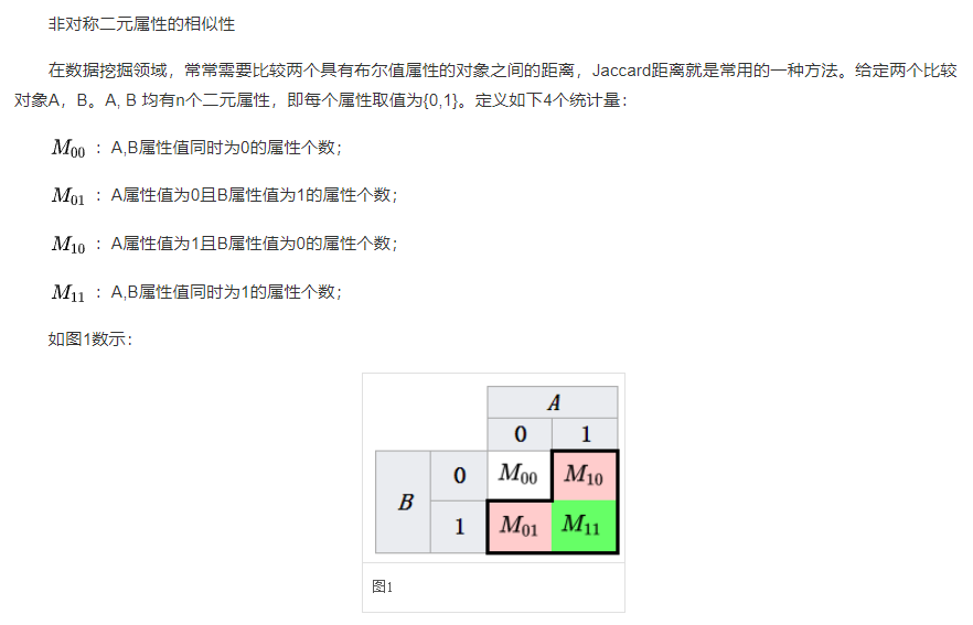
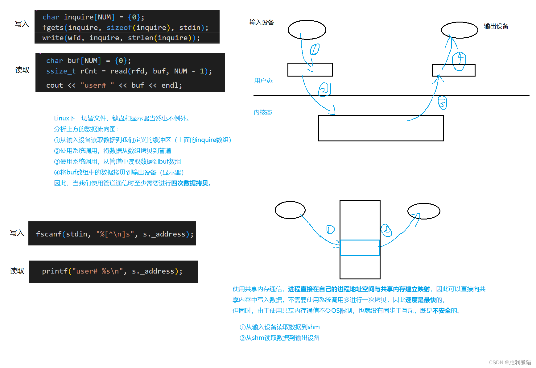
文章目录
- brief
- KNN(k-nearest neighbor)简介部分
- SNN(shared nearest neighbor)简介部分
- Annoy算法理解
- Jaccard index
- Seurat进行聚类的步骤
- 可视化部分
- subcluster之间的marker gene
- 具体参数
brief
seurat 官方教程的解释如下:
- 大概是第一步利用PCA降维结果作为input,计算euclidean distance从而构建KNN graph,然后根据两两细胞间的Jaccard similarity 重新构建SNN graph。
- 第二步 partition this graph
==================================================================================
KNN(k-nearest neighbor)简介部分
- 上面的描述可以认为是KNN的原理或者思想。
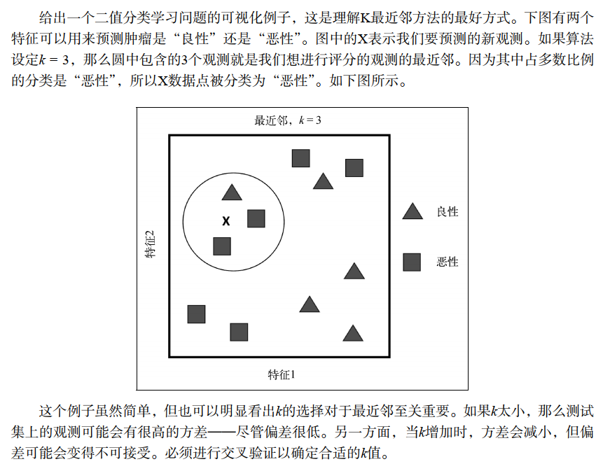
- 我们需要关注的是如何快速从数据集中找到和目标样本最接近的K个样本?
如果数据量很小,我们可以根据距离度量公式计算一个距离度量表,然后排序后筛选K个最近邻。如果数据量很大,再计算每个数据点的距离会很耗费资源,所以需要特殊的实现方法以节省资源,比如KDtree,Annoy等。
================================================================================
SNN(shared nearest neighbor)简介部分
下面的内容来自博客:
原文链接:https://blog.csdn.net/qq_40793975/article/details/84817018
共享最近邻相似度(Shared Nearest Neighbour,简称SNN)基于这样一个事实,如果两个点都与一些相同的点相似,则即使直接的相似性度量不能指出,他们也相似,更具体地说,只要两个对象都在对方的最近邻表中,SNN相似度就是他们共享的近邻个数,计算过程如下图所示。需要注意的是,这里用来获取最近邻表时所使用的邻近性度量可以是任何有意义的相似性或相异性度量。

下面通过一个实例进行直观的说明,假设两个对象A、B(黑色的)都有8个最近邻,且这两个对象之间相互包含,这些最近邻中有4个(灰色的)是A、B共享的,因此这两个对象之间的SNN相似度为4。

对象之间SNN相似度的相似度图称作SNN相似度图(SNN similarity graph),由于许多对象之间的SNN相似度为0,因此SNN相似度图非常稀疏。
SNN相似度解决了使用直接相似度时出现的一些问题,首先,他可以处理如下情况,一个对象碰巧与另一个对象相对较近,但是两者分属于不同的簇,由于在这种情况下,两个对象一般不包含许多的共享近邻,因此他们的SNN密度很低。另一种情况是,当处理不同密度的簇时,由于一对对象之间的相似度不依赖于两者之间的距离,而是两者的共享近邻,因此SNN密度会根据簇的密度进行合适的伸缩。
=================================================================================
Annoy算法理解
这里推荐一篇知乎。
个人认为这里只需要简单知道 what’s that ? what to do ?
- 是什么?
一种数据的存储和搜索方法 - 干什么?
利用特殊的数据储存和搜索方法实现快速的返回 Top K 相似的数据
=================================================================================
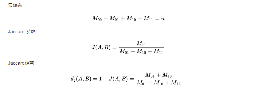
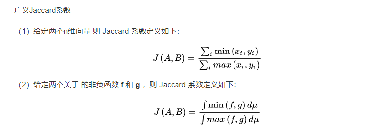
Jaccard index
下面的内容来自百度百科:
Jaccard index , 又称为Jaccard相似系数(Jaccard similarity coefficient)用于比较有限样本集之间的相似性与差异性。Jaccard系数值越大,样本相似度越高。

Seurat进行聚类的步骤
pbmc <- FindNeighbors(pbmc, dims = 1:10)
pbmc <- FindClusters(pbmc, resolution = 0.5)
================================================================================
可视化部分
- UMAP非线性降维
# If you haven't installed UMAP, you can do so via reticulate::py_install(packages =
# 'umap-learn')
pbmc <- RunUMAP(pbmc, dims = 1:10)
# note that you can set `label = TRUE` or use the LabelClusters function to help label
# individual clusters
DimPlot(pbmc, reduction = "umap")
- marker gene 可视化部分
# 小提琴图
VlnPlot(pbmc, features = c("MS4A1", "CD79A"))
# 山脊图
RidgePlot(object = pbmc_small, features = 'PC_1')
# 散点图
CellScatter(object = pbmc_small, cell1 = 'ATAGGAGAAACAGA', cell2 = 'CATCAGGATGCACA')
# 气泡图
cd_genes <- c("CD247", "CD3E", "CD9")
DotPlot(object = pbmc_small, features = cd_genes)
# feature plot
FeaturePlot(pbmc, features = c("MS4A1", "GNLY", "CD3E", "CD14", "FCER1A", "FCGR3A", "LYZ", "PPBP",
    "CD8A"))
subcluster之间的marker gene
# find all markers of cluster 2
cluster2.markers <- FindMarkers(pbmc, ident.1 = 2, min.pct = 0.25)
head(cluster2.markers, n = 5)

# find all markers distinguishing cluster 5 from clusters 0 and 3
cluster5.markers <- FindMarkers(pbmc, ident.1 = 5, ident.2 = c(0, 3), min.pct = 0.25)
head(cluster5.markers, n = 5)

# find markers for every cluster compared to all remaining cells, report only the positive
# ones
pbmc.markers <- FindAllMarkers(pbmc, only.pos = TRUE, min.pct = 0.25, logfc.threshold = 0.25)
pbmc.markers %>%
    group_by(cluster) %>%
    slice_max(n = 2, order_by = avg_log2FC)

# Seurat has several tests for differential expression which can be set with the test.use parameter
# For example, the ROC test returns the ‘classification power’ for any individual marker (ranging from 0 - random, to 1 - perfect)
cluster0.markers <- FindMarkers(pbmc, ident.1 = 0, logfc.threshold = 0.25, test.use = "roc", only.pos = TRUE)
=================================================================================
具体参数
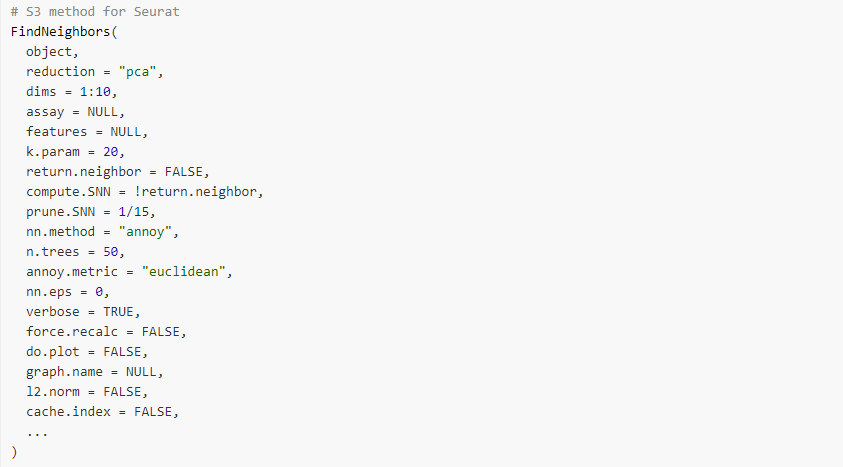
-
k.param
Defines k for the k-nearest neighbor algorithm
这里最想说的是K为什么不设为奇数而是设为偶数~~ -
return.neighbor
Return result as Neighbor object. Not used with distance matrix input. -
compute.SNN
also compute the shared nearest neighbor graph -
prune.SNN
Sets the cutoff for acceptable Jaccard index when computing the neighborhood overlap for the SNN construction. Any edges with values less than or equal to this will be set to 0 and removed from the SNN graph. Essentially sets the stringency of pruning (0 — no pruning, 1 — prune everything). -
nn.method
Method for nearest neighbor finding. Options include: rann, annoy -
n.trees
More trees gives higher precision when using annoy approximate nearest neighbor search -
annoy.metric
Distance metric for annoy. Options include: euclidean, cosine, manhattan, and hamming -
nn.eps
Error bound when performing nearest neighbor seach using RANN; default of 0.0 implies exact nearest neighbor search -
verbose
Whether or not to print output to the console -
force.recalc
Force recalculation of (S)NN. -
l2.norm
Take L2Norm of the data -
cache.index
Include cached index in returned Neighbor object (only relevant if return.neighbor = TRUE) -
index
Precomputed index. Useful if querying new data against existing index to avoid recomputing. -
features
Features to use as input for building the (S)NN; used only when dims is NULL -
reduction
Reduction to use as input for building the (S)NN -
dims
Dimensions of reduction to use as input -
assay
Assay to use in construction of (S)NN; used only when dims is NULL -
do.plot
Plot SNN graph on tSNE coordinates -
graph.name
Optional naming parameter for stored (S)NN graph (or Neighbor object, if return.neighbor = TRUE). Default is assay.name_(s)nn. To store both the neighbor graph and the shared nearest neighbor (SNN) graph, you must supply a vector containing two names to the graph.name parameter. The first element in the vector will be used to store the nearest neighbor (NN) graph, and the second element used to store the SNN graph. If only one name is supplied, only the NN graph is stored

-
modularity.fxn
Modularity function (1 = standard; 2 = alternative). -
initial.membership, node.sizes
Parameters to pass to the Python leidenalg function. -
resolution
Value of the resolution parameter, use a value above (below) 1.0 if you want to obtain a larger (smaller) number of communities. -
method
Method for running leiden (defaults to matrix which is fast for small datasets). Enable method = “igraph” to avoid casting large data to a dense matrix. -
algorithm
Algorithm for modularity optimization (1 = original Louvain algorithm; 2 = Louvain algorithm with multilevel refinement; 3 = SLM algorithm; 4 = Leiden algorithm). Leiden requires the leidenalg python. -
n.start
Number of random starts. -
n.iter
Maximal number of iterations per random start. -
random.seed
Seed of the random number generator. -
group.singletons
Group singletons into nearest cluster. If FALSE, assign all singletons to a “singleton” group -
temp.file.location
Directory where intermediate files will be written. Specify the ABSOLUTE path. -
edge.file.name
Edge file to use as input for modularity optimizer jar. -
verbose
Print output -
graph.name
Name of graph to use for the clustering algorithm


![[学习笔记] [机器学习] 4. [下]线性回归(正规方程、梯度下降、岭回归)](https://img-blog.csdnimg.cn/bc773cd7b94f4a9f93a484e5e7c7ce0c.png#pic_center)