VGG网络实现：https://blog.csdn.net/weixin_43912621/article/details/127852595
论文地址：https://arxiv.org/abs/1409.1556

VERY DEEP CONVOLUTIONAL NETWORKS FOR LARGE-SCALE IMAGE RECOGNITION

用于大规模图像识别的深度卷积网络

Abstract

In this work we investigate the effect of the convolutional network depth on its accuracy in the large-scale image recognition setting. Our main contribution is a thorough evaluation of networks of increasing depth using an architecture with very small (3 × 3) convolution filters, which shows that a significant improvement on the prior-art configurations can be achieved by pushing the depth to 16–19 weight layers. These findings were the basis of our ImageNet Challenge 2014 submission, where our team secured the first and the second places in the localisation and classification tracks respectively. We also show that our representations generalise well to other datasets, where they achieve state-of-the-art results. We have made our two best-performing ConvNet models publicly available to facili-tate further research on the use of deep visual representations in computer vision.

在这项工作中，我们研究了卷积网络深度对其在大规模图像识别设置中的准确性的影响。在这项工作中，我们研究了卷积网络深度对其在大规模图像识别设置中的准确性的影响。我们的主要贡献是使用非常小(3 × 3)卷积滤波器的架构对深度增加的网络进行了全面评估，这表明了通过将深度推至16-19个权重层，可以实现对现有技术配置的显著改进。这些发现是我们提交2014 ImageNet挑战赛的基础，我们的团队分别在本地化和分类赛道上获得了第一和第二名。我们还表明，我们的发现可以很好地推广到其他数据集，在这些数据集中，它们实现了最先进的结果。我们已经公开了两个性能最好的ConvNet模型，以促进在计算机视觉中使用深度视觉表示的进一步研究。

1 INTRODUCTION

Convolutional networks (ConvNets) have recently enjoyed a great success in large-scale image and video recognition (Krizhevsky et al., 2012; Zeiler & Fergus, 2013; Sermanet et al., 2014;Simonyan & Zisserman, 2014) which has become possible due to the large public image repositories, such as ImageNet (Deng et al., 2009), and high-performance computing systems, such as GPUs or large-scale distributed clusters (Dean et al., 2012). In particular, an important role in the advance of deep visual recognition architectures has been played by the ImageNet Large-Scale Visual Recognition Challenge (ILSVRC) (Russakovsky et al., 2014), which has served as a testbed for a few generations of large-scale image classification systems, from high-dimensional shallow feature encodings (Perronnin et al., 2010) (the winner of ILSVRC-2011) to deep ConvNets (Krizhevsky et al.,2012) (the winner of ILSVRC-2012).

卷积网络(ConvNets)最近在大规模图像和视频识别方面取得了巨大成功(Krizhevsky等人，2012；Zeiler & Fergus, 2013；Sermanet et al.， 2014；Simonyan & Zisserman, 2014)，由于大型公共图像存储库，如ImageNet(Deng等人，2009)和高性能计算系统，如gpu或大规模分布式集群(Dean等人，2012)，这已经成为可能。特别是，ImageNet大规模视觉识别挑战(ILSVRC) (Russakovsky等人，2014年)在深度视觉识别体系结构的发展中发挥了重要作用，它已作为几代大规模图像分类系统的测试平台，从高维浅特征编码(Perronnin等人，2010年)(ILSVRC -2011年的获胜者)到深度ConvNets (Krizhevsky等人，2012年)(ILSVRC -2012年的获胜者)。

With ConvNets becoming more of a commodity in the computer vision field, a number of attempts have been made to improve the original architecture of Krizhevsky et al. (2012) in a bid to achieve better accuracy. For instance, the best-performing submissions to the ILSVRC2013 (Zeiler & Fergus，2013；Sermanet et al.，2014) utilised smaller receptive window size and smaller stride of the first convolutional layer. Another line of improvements dealt with training and testing the networks densely over the whole image and over multiple scales (Sermanet et al., 2014；Howard，2014). In this paper, we address another important aspect of ConvNet architecture design – its depth. To this end, we fix other parameters of the architecture, and steadily increase the depth of the network by adding more convolutional layers, which is feasible due to the use of very small (3 × 3) convolution filters in all layers.

随着ConvNets越来越成为计算机视觉领域的必需品，人们尝试改进Krizhevsky等人(2012)的原始架构，以获得更好的精度。例如，ILSVRC2013 最好表现的提交(Zeiler & Fergus，2013；Sermanet et al.， 2014)利用了更小的接受窗口大小和更小的第一卷积层步幅。另一项改进涉及在整个图像和多个尺度上密集地训练和测试网络(Sermanet et al.， 2014；Doward，2014)。在本文中，我们讨论了ConvNet体系结构设计的另一个重要方面——深度。为此，我们固定了架构的其他参数，并通过增加更多的卷积层来稳步增加网络的深度，这是可行的，因为在所有层中都使用了非常小的(3 × 3)卷积滤波器。

As a result, we come up with significantly more accurate ConvNet architectures, which not only achieve the state-of-the-art accuracy on ILSVRC classification and localisation tasks, but are also applicable to other image recognition datasets, where they achieve excellent performance even when used as a part of a relatively simple pipelines (e.g. deep features classified by a linear SVM without fine-tuning). We have released our two best-performing models1 to facilitate further research.

因此，我们提出了更精确的ConvNet体系结构，不仅在ILSVRC分类和定位任务上实现了最先进的精度，而且也适用于其他图像识别数据集，即使作为相对简单管道的一部分(例如，在没有微调的情况下由线性SVM分类的深度特征)，它们也能获得出色的性能。我们已经发布了两个性能最好的模型，以促进进一步的研究。

The rest of the paper is organised as follows. In Sect. 2, we describe our ConvNet configurations.The details of the image classification training and evaluation are then presented in Sect. 3. The configurations are compared on the ILSVRC classification task in Sect. 4. Sect. 5 concludes the paper. For completeness, we also describe and assess our ILSVRC-2014 object localisation system in Appendix A, and discuss the generalisation of very deep features to other datasets in Appendix B.Finally, Appendix C contains the list of major paper revisions.

本文的其余部分组织如下。在第2节中，我们描述了ConvNet的配置。然后在第3节中介绍了图像分类训练和评估的细节。在第4节的ILSVRC分类任务中比较配置。第五节对全文进行了总结。为了完整起见，我们还在附录A中描述和评估了我们的ILSVRC-2014对象定位系统，并在附录B中讨论了非常深入的特征对其他数据集的概括。最后，附录C包含了主要论文修订的列表。

2 CONVNET CONFIGURATIONS

To measure the improvement brought by the increased ConvNet depth in a fair setting, all our ConvNet layer configurations are designed using the same principles, inspired by Ciresan et al(2011); Krizhevsky et al (2012). In this section, we first describe a generic layout of our ConvNet configurations (Sect. 2.1) and then detail the specific configurations used in the evaluation (Sect. 2.2).Our design choices are then discussed and compared to the prior art in Sect. 2.3.

为了衡量在公平环境下增加ConvNet深度所带来的改进，我们所有的ConvNet层配置都使用相同的原理设计，灵感来自Ciresan等人(2011)；Krizhevsky et al(2012)。在本节中，我们首先描述ConvNet配置的一般布局(第2.1节)，然后详细介绍评估中使用的具体配置(第2.2节)。然后我们的设计选择，并与第2.3节中的现有技术进行比较。

2.1 ARCHITECTURE

During training, the input to our ConvNets is a fixed-size 224 × 224 RGB image. The only preprocessing we do is subtracting the mean RGB value, computed on the training set, from each pixel.The image is passed through a stack of convolutional (conv.) layers, where we use filters with a very small receptive field: 3 × 3 (which is the smallest size to capture the notion of left/right, up/down, center). In one of the configurations we also utilise 1 × 1 convolution filters, which can be seen as a linear transformation of the input channels (followed by non-linearity). The convolution stride is fixed to 1 pixel; the spatial padding of conv. layer input is such that the spatial resolution is preserved after convolution, i.e. the padding is 1 pixel for 3 × 3 conv. layers. Spatial pooling is carried out by five max-pooling layers, which follow some of the conv. layers (not all the conv. layers are followed by max-pooling). Max-pooling is performed over a 2 × 2 pixel window, with stride 2.

在训练过程中，ConvNets的输入是一个固定大小的224 × 224 RGB图像。我们所做的唯一预处理是从每个像素中减去在训练集上计算的平均RGB值。图像经过一堆卷积(conv.)层，其中我们使用一个非常小的接受域过滤器:3 × 3(这是捕获左/右、上/下、中心概念的最小尺寸)。在其中一种配置中，我们还使用了1 × 1卷积滤波器，它可以被视为输入通道的线性变换(其次是非线性)。卷积步幅固定为1像素;卷积层输入的空间填充使卷积后的空间分辨率保持不变，即3 × 3个卷积层的填充为1像素。空间池化是由5个max-pooling层执行的，它们跟随在一些convl .层之后(并不是所有convl .层之后都跟随max-pooling层)。最大池化在2 × 2像素的窗口上执行，步幅为2。

A stack of convolutional layers (which has a different depth in different architectures) is followed by three Fully-Connected (FC) layers: the first two have 4096 channels each, the third performs 1000way ILSVRC classification and thus contains 1000 channels (one for each class). The final layer is the soft-max layer. The configuration of the fully connected layers is the same in all networks.

卷积层的堆栈(在不同的体系结构中有不同的深度)后面是三个全连接(FC)层:前两个层各有4096个通道，第三个层执行1000way ILSVRC分类，因此包含1000个通道(每个类一个)。最后一层是soft-max层。全连接层的配置在所有网络中都是相同的。

All hidden layers are equipped with the rectification (ReLU (Krizhevsky et al, 2012)) non-linearity.We note that none of our networks (except for one) contain Local Response Normalisation (LRN) normalisation (Krizhevsky et al, 2012): as will be shown in Sect. 4, such normalisation does not improve the performance on the ILSVRC dataset, but leads to increased memory consumption and computation time. Where applicable, the parameters for the LRN layer are those of (Krizhevsky et al, 2012).

所有隐藏层都装备有ReLU函数 (Krizhevsky et al, 2012)非线性。我们注意到，我们的网络(除了一个)都没有包含局部响应归一化(LRN)归一化(Krizhevsky等人，2012):正如第4节所示，这种归一化不会提高ILSVRC数据集上的性能，但会导致内存消耗和计算时间的增加。在适用的情况下，LRN层的参数为(Krizhevsky et al, 2012)。

2.2 CONFIGURATIONS

The ConvNet configurations, evaluated in this paper, are outlined in Table 1, one per column. In the following we will refer to the nets by their names (A–E). All configurations follow the generic design presented in Sect. 2.1, and differ only in the depth: from 11 weight layers in the network A (8 conv. and 3 FC layers) to 19 weight layers in the network E (16 conv. and 3 FC layers). The width of conv. layers (the number of channels) is rather small, starting from 64 in the first layer and then increasing by a factor of 2 after each max-pooling layer, until it reaches 512.

本文中评估的ConvNet配置在表1中列出，每列一个。在下文中，我们将按网的名称(A-E)来表示。所有的配置都遵循2.1节中给出的通用设计，仅在深度上有所不同:从网络A的11个权重层(8节和3层FC)到网络E的19个权重层(16节和3层FC)。convc . layers的宽度(通道数量)相当小，从第一层的64开始，然后在每个max-pooling层后增加2倍，直到达到512。

2.3 DISCUSSION

Our ConvNet configurations are quite different from the ones used in the top-performing entries of the ILSVRC-2012 (Krizhevsky et al, 2012) and ILSVRC-2013 competitions (Zeiler & Fergus, 2013; Sermanet et al, 2014). Rather than using relatively large receptive fields in the first conv. layers (e.g. 11×11 with stride 4 in (Krizhevsky et al, 2012), or 7×7 with stride 2 in (Zeiler & Fergus, 2013; Sermanet et al, 2014)), we use very small 3 × 3 receptive fields throughout the whole net, which are convolved with the input at every pixel (with stride 1). It is easy to see that a stack of two 3×3 conv. layers (without spatial pooling in between) has an effective receptive field of 5×5; three such layers have a 7 x 7 effective receptive field.So what have we gained by using,for instance,a stack of three 3 x 3 conv.layers instead of a single 7 x 7 layer?First,we incorporate three non-linear rectification layers instead of a single one,which makes the decision function more discriminative. Second,we decrease the number of parameters:assuming that both the input and the output of a three-layer 3 x 3 convolution stack has C channels,the stack is parametrised by 3(3²C²)=27C² weights;at the same time,a single 7x 7 conv.layer would require 7²C² =49C² parameters,i.e. 81%more.This can be seen as imposing a regularisation on the 7 x 7 conv.filters,forcing them to have a decomposition through the 3 x 3 filters(with non-linearity injected in between).

我们的ConvNet配置与在ILSVRC-2012 (Krizhevsky等人，2012)和ILSVRC-2013比赛(Zeiler & Fergus, 2013;Sermanet et al, 2014)中表现最好的不同。我们抛弃在第一个conv.层中使用相对较大的接受域(例如，11×11与stride 4 in (Krizhevsky et al, 2012)，或7×7与stride 2 in (Zeiler & Fergus, 2013;(Sermanet et al, 2014))，而是在整个网络中使用非常小的3×3接受域，在每个像素处与输入进行卷积(stride为1)。很容易看到两个3×3 convl .层的堆栈(中间没有空间池化)具有5×5的有效接受域;三个这种层具有7 × 7的有效感受野。那么，通过使用三个3×3 convc .层而不是一个7×7层，我们得到了什么呢?首先，我们引入三个非线性校正层，而不是单一校正层，使决策函数更具辨识性;其次，我们减少了参数的数量:假设一个三层3 × 3卷积堆栈的输入和输出都有C通道，堆栈参数化为3 (3²C²) = 27c²权值；同时，单个7 × 7 conv.层需要7²C² = 49c²参数，即多出81%。这可以看作是对7 × 7 convl .滤波器施加了正则化，迫使它们通过3 × 3滤波器进行分解(在两者之间注入非线性)。

The incorporation of 1 × 1 conv. layers (configuration C, Table 1) is a way to increase the nonlinearity of the decision function without affecting the receptive fields of the conv. layers. Even though in our case the 1 × 1 convolution is essentially a linear projection onto the space of the same dimensionality (the number of input and output channels is the same), an additional non-linearity is introduced by the rectification function. It should be noted that 1×1 conv. layers have recently been utilised in the “Network in Network” architecture of Lin et al (2014).

1 × 1 conv. layers的合并(配置C，表1)是一种增加决策函数的非线性而不影响conv. layers的接受场的方法。尽管在我们的例子中，1 × 1卷积本质上是在相同维度的空间上的线性投影(输入和输出通道的数量相同)，但校正函数引入了额外的非线性。值得注意的是，1×1 convc . layers最近被用于Lin等人(2014)的“网络中的网络”体系结构。

在这里插入图片描述

Small-size convolution filters have been previously used by Ciresan et al (2011), but their nets are significantly less deep than ours, and they did not evaluate on the large-scale ILSVRC dataset. Goodfellow et al (2014) applied deep ConvNets (11 weight layers) to the task of street number recognition, and showed that the increased depth led to better performance.GoogLeNet (Szegedy et al, 2014), a top-performing entry of the ILSVRC-2014 classification task, was developed independently of our work, but is similar in that it is based on very deep ConvNets
(22 weight layers) and small convolution filters (apart from 3 × 3, they also use 1 × 1 and 5 × 5 convolutions). Their network topology is, however, more complex than ours, and the spatial resolution of the feature maps is reduced more aggressively in the first layers to decrease the amount of computation. As will be shown in Sect. 4.5, our model is outperforming that of Szegedy et al(2014) in terms of the single-network classification accuracy.

Ciresan等人（2011）以前使用过小尺寸的卷积滤波器，但他们的网络比我们的网络要浅得多，并且他们没有在大规模的ILSVRC数据集上进行评估。Goodfellow等人（2014）将深度ConvNet（11个权重层）应用于街道数字识别任务，并显示增加的深度导致更好的性能。GoogLeNet（Szegedy等人，2014）是ILSVRC-2014分类任务的最佳表现之一，独立于我们的工作开发，但类似于我们的工作，基于非常深的ConvNet（22个权重层）和小卷积滤波器（除了3×3之外，他们还使用1×1和5×5的卷积）。然而，他们的网络拓扑比我们的更加复杂，并且在第一层中更积极地减少了特征图的空间分辨率以减少计算量。如第4.5节所示，我们的模型在单网络分类准确性方面表现优于Szegedy等人（2014）的模型。

3 CLASSIFICATION FRAMEWORK

In the previous section we presented the details of our network configurations. In this section, we describe the details of classification ConvNet training and evaluation.

在前一节中，我们介绍了网络配置的详细信息。在本节中，我们描述了分类ConvNet训练和评估的细节。

3.1 TRAINING

The ConvNet training procedure generally follows Krizhevsky et al (2012) (except for sampling the input crops from multi-scale training images, as explained later). Namely, the training is carried out by optimising the multinomial logistic regression objective using mini-batch gradient descent (based on back-propagation (LeCun et al, 1989)) with momentum. The batch size was set to 256, momentum to 0.9. The training was regularised by weight decay (the L2 penalty multiplier set to 5 · 10⁻⁴ ) and dropout regularisation for the first two fully-connected layers (dropout ratio set to 0.5).The learning rate was initially set to 10⁻² , and then decreased by a factor of 10 when the validation set accuracy stopped improving. In total, the learning rate was decreased 3 times, and the learning was stopped after 370K iterations (74 epochs). We conjecture that in spite of the larger number of parameters and the greater depth of our nets compared to (Krizhevsky et al, 2012), the nets required less epochs to converge due to (a) implicit regularisation imposed by greater depth and smaller conv.filter sizes; (b) pre-initialisation of certain layers.

这个卷积神经网络的训练过程基本上遵循Krizhevsky等人（2012）的方法（除了后面解释的从多尺度训练图像中采样输入样本的步骤）。具体来说，我们通过使用动量（momentum）的小批量梯度下降法（基于反向传播（LeCun等人，1989））来优化多项式逻辑回归目标进行训练。批次大小设置为256，动量为0.9。训练通过权重衰减（L2惩罚因子设置为5×10⁻⁴）和dropout正则化（对于前两个全连接层，dropout比例设置为0.5）进行规范化。学习率最初设置为10⁻²，当验证集准确率停止提高时，将其降低10倍。总共降低了3次学习率，在370K次迭代（74个epochs）后停止学习。我们猜测，尽管我们的神经网络的参数更多，深度更大，但由于（a）更大的深度和更小的卷积滤波器大小所施加的隐式正则化;（b）对某些层的预初始化，我们的网络收敛所需的迭代次数更少。

The initialisation of the network weights is important, since bad initialisation can stall learning due to the instability of gradient in deep nets. To circumvent this problem, we began with training the configuration A (Table 1), shallow enough to be trained with random initialisation. Then, when training deeper architectures, we initialised the first four convolutional layers and the last three fullyconnected layers with the layers of net A (the intermediate layers were initialised randomly). We did not decrease the learning rate for the pre-initialised layers, allowing them to change during learning.For random initialisation (where applicable), we sampled the weights from a normal distribution with the zero mean and 10⁻² variance. The biases were initialised with zero. It is worth noting that after the paper submission we found that it is possible to initialise the weights without pre-training by using the random initialisation procedure of Glorot & Bengio (2010)

网络权重的初始化很重要，因为糟糕的初始化可能会导致梯度不稳定而阻碍深度网络的学习。为了避免这个问题，我们首先训练配置A（表1），它足够浅，可以使用随机初始化进行训练。然后，在训练更深的体系结构时，我们使用网络A的前四个卷积层和最后三个全连接层来初始化它们（中间层随机初始化）。我们没有降低预初始化层的学习率，允许它们在学习过程中发生变化。对于随机初始化（适用时），我们从零均值和10⁻²方差的正态分布中采样权重。偏差初始化为零。值得注意的是，在提交论文后，我们发现可以通过使用Glorot＆Bengio（2010）的随机初始化程序来初始化权重。

To obtain the fixed-size 224×224 ConvNet input images, they were randomly cropped from rescaled training images (one crop per image per SGD iteration). To further augment the training set, the crops underwent random horizontal flipping and random RGB colour shift (Krizhevsky et al, 2012).Training image rescaling is explained below.

为了得到固定尺寸的 224×224 的 ConvNet 输入图像，它们是从经过缩放的训练图像中随机裁剪得到的（每次 SGD 迭代每张图像裁剪一次）。为了进一步增加训练集，这些裁剪图像会经过随机水平翻转和随机 RGB 颜色变换（Krizhevsky et al，2012）。训练图像的缩放将在下面进行解释。

Training image size. Let S be the smallest side of an isotropically-rescaled training image, from which the ConvNet input is cropped (we also refer to S as the training scale). While the crop size is fixed to 224 × 224, in principle S can take on any value not less than 224: for S = 224 the crop will capture whole-image statistics, completely spanning the smallest side of a training image; for S ≫ 224 the crop will correspond to a small part of the image, containing a small object or an object part.

**训练图像大小。**设S为等比缩放的训练图像的最小边，从中裁剪ConvNet输入（我们也称S为训练尺度）。虽然裁剪大小固定为224×224，但原则上S可以取任何不小于224的值：对于S = 224，裁剪将捕捉整个图像的统计信息，完全跨越训练图像的最小边；对于S ≫ 224，裁剪将对应于图像的一小部分，包含小物体或物体的一部分。

We consider two approaches for setting the training scale S. The first is to fix S, which corresponds to single-scale training (note that image content within the sampled crops can still represent multiscale image statistics). In our experiments, we evaluated models trained at two fixed scales: S = 256 (which has been widely used in the prior art (Krizhevsky et al, 2012; Zeiler & Fergus, 2013; Sermanet et al, 2014)) and S = 384. Given a ConvNet configuration, we first trained the network using S = 256. To speed-up training of the S = 384 network, it was initialised with the weights pre-trained with S = 256, and we used a smaller initial learning rate of 10⁻³ .

我们考虑两种方法来设置训练尺度S。第一种方法是固定S，这对应于单尺度训练（注意，采样裁剪内的图像内容仍然可以代表多尺度图像统计信息）。在我们的实验中，我们评估了在两个固定尺度S下训练的模型：S = 256（这在先前的研究中已被广泛使用（Krizhevsky et al，2012; Zeiler＆Fergus，2013; Sermanet et al，2014））和S = 384。给定一个ConvNet配置，我们首先使用S = 256训练网络。为了加快S = 384网络的训练速度，我们使用了在S = 256下预训练的权重来初始化网络，并使用了较小的初始学习率10⁻³。

The second approach to setting S is multi-scale training, where each training image is individually rescaled by randomly sampling S from a certain range [Smin, Smax] (we used Smin = 256 and Smax = 512). Since objects in images can be of different size, it is beneficial to take this into account during training. This can also be seen as training set augmentation by scale jittering, where a single model is trained to recognise objects over a wide range of scales. For speed reasons, we trained multi-scale models by fine-tuning all layers of a single-scale model with the same configuration, pre-trained with fixed S = 384.

第二种设置S的方法是多尺度训练，其中每个训练图像通过从某个范围[Smin，Smax]中随机采样S来单独重新调整大小（我们使用Smin = 256和Smax = 512）。由于图像中的对象可能具有不同的尺寸，因此在训练期间考虑这一点是有益的。这也可以看作是通过尺度抖动的训练集增强，其中单个模型被训练以在各种尺度范围内识别对象。由于速度原因，我们通过微调具有相同配置的单尺度模型的所有层来训练多尺度模型，该单尺度模型使用S = 384的固定尺度预先训练。

3.2 TESTING

At test time, given a trained ConvNet and an input image, it is classified in the following way. First, it is isotropically rescaled to a pre-defined smallest image side, denoted as Q (we also refer to it as the test scale). We note that Q is not necessarily equal to the training scale S (as we will show in Sect. 4, using several values of Q for each S leads to improved performance). Then, the network is applied densely over the rescaled test image in a way similar to (Sermanet et al, 2014). Namely, the fully-connected layers are first converted to convolutional layers (the first FC layer to a 7 × 7 conv. layer, the last two FC layers to 1 × 1 conv. layers). The resulting fully-convolutional net is then applied to the whole (uncropped) image. The result is a class score map with the number of channels equal to the number of classes, and a variable spatial resolution, dependent on the input image size. Finally, to obtain a fixed-size vector of class scores for the image, the class score map is spatially averaged (sum-pooled). We also augment the test set by horizontal flipping of the images; the soft-max class posteriors of the original and flipped images are averaged to obtain the final scores for the image.

在测试时，给定一个经过训练的 ConvNet 和一个输入图像，按照以下方式进行分类。首先，它被等比例地缩放到预定义的最小图像边界，称为 Q（我们也将其称为测试尺度）。我们注意到 Q 不一定等于训练尺度 S（正如我们将在第 4 节中展示的，为每个 S 使用几个 Q 的值可以提高性能）。然后，网络以类似于（Sermanet et al，2014）的方式在经过缩放的测试图像上密集地应用。即，首先将全连接层转换为卷积层（第一个 FC 层为 7×7 的卷积层，最后两个 FC 层为 1×1 的卷积层）。然后，将结果完全卷积网络应用于整个（未裁剪的）图像。结果是一个类得分映射，其通道数等于类的数量，并且具有可变的空间分辨率，这取决于输入图像的大小。最后，为了获得图像的固定大小的类得分向量，对类得分映射进行空间平均（求和池化）。我们还通过水平翻转图像来增强测试集；对原始图像和翻转图像的soft-max后平均以获得图像的最终得分。

Since the fully-convolutional network is applied over the whole image, there is no need to sample multiple crops at test time (Krizhevsky et al, 2012), which is less efficient as it requires network re-computation for each crop. At the same time, using a large set of crops, as done by Szegedy et al(2014), can lead to improved accuracy, as it results in a finer sampling of the input image compared to the fully-convolutional net. Also, multi-crop evaluation is complementary to dense evaluation due to different convolution boundary conditions: when applying a ConvNet to a crop, the convolved feature maps are padded with zeros, while in the case of dense evaluation the padding for the same crop naturally comes from the neighbouring parts of an image (due to both the convolutions and spatial pooling), which substantially increases the overall network receptive field, so more context is captured. While we believe that in practice the increased computation time of multiple crops does not justify the potential gains in accuracy, for reference we also evaluate our networks using 50 crops per scale (5 × 5 regular grid with 2 flips), for a total of 150 crops over 3 scales, which is comparable to 144 crops over 4 scales used by Szegedy et al (2014).

由于完全卷积网络是在整个图像上应用的，因此在测试时无需对多个裁剪进行采样（Krizhevsky等人，2012），因为这会导致每个裁剪需要重新计算网络，效率较低。同时，使用大量的裁剪，如Szegedy等人（2014）所做的，可以提高准确性，因为相对于完全卷积网络，它可以对输入图像进行更细致的采样。此外，由于卷积边界条件不同，多裁剪评估对于密集评估是互补的：在将ConvNet应用于裁剪时，卷积特征图会用零进行填充，而在密集评估的情况下，同一裁剪的填充自然来自图像的邻近部分（由于卷积和空间池化），这大大增加了整个网络的接受域，从而捕获更多的上下文信息。虽然我们认为在实践中，多个裁剪所需的计算时间不足以证明准确性的潜在收益，但是为了参考，我们也使用每个区域50个裁剪（5×5个常规网格，翻转2次）来评估我们的网络，总共在3个区域上使用了150个裁剪，这与Szegedy等人（2014）使用的4个区域上的144个裁剪相当。

3.3 IMPLEMENTATION DETAILS

Our implementation is derived from the publicly available C++ Caffe toolbox (Jia, 2013) (branched out in December 2013), but contains a number of significant modifications, allowing us to perform training and evaluation on multiple GPUs installed in a single system, as well as train and evaluate on full-size (uncropped) images at multiple scales (as described above). Multi-GPU training exploits data parallelism, and is carried out by splitting each batch of training images into several GPU batches, processed in parallel on each GPU. After the GPU batch gradients are computed, they are averaged to obtain the gradient of the full batch. Gradient computation is synchronous across the GPUs, so the result is exactly the same as when training on a single GPU.

我们的实现基于公开可用的C++ Caffe工具箱（Jia，2013）（在2013年12月分支出），但包含了许多重要的修改，使我们能够在单个系统上安装的多个GPU上执行训练和评估，以及在多个尺度上对完整大小（未裁剪）的图像进行训练和评估（如上所述）。多GPU训练利用数据并行性，并通过将每个训练图像批次分成几个GPU批次来在每个GPU上并行处理。计算GPU批次梯度后，它们被平均以获得整个批次的梯度。梯度计算在GPU之间同步，因此结果与在单个GPU上训练时完全相同。

While more sophisticated methods of speeding up ConvNet training have been recently proposed (Krizhevsky, 2014), which employ model and data parallelism for different layers of the net, we have found that our conceptually much simpler scheme already provides a speedup of 3.75 times on an off-the-shelf 4-GPU system, as compared to using a single GPU. On a system equipped with four NVIDIA Titan Black GPUs, training a single net took 2–3 weeks depending on the architecture.

虽然最近已经提出了更复杂的加速ConvNet训练的方法（Krizhevsky, 2014），其中利用模型和数据并行化来处理网络的不同层，但我们发现，我们这个概念上更简单的方案已经在一台配备了4个GPU的现成系统上实现了3.75倍的加速，相对于使用单个GPU。在配备了四个NVIDIA Titan Black GPU的系统上，训练单个网络需要2-3周，具体时间取决于网络的架构。

4 CLASSIFICATION EXPERIMENTS

Dataset. In this section, we present the image classification results achieved by the described ConvNet architectures on the ILSVRC-2012 dataset (which was used for ILSVRC 2012–2014 challenges). The dataset includes images of 1000 classes, and is split into three sets: training (1.3M images), validation (50K images), and testing (100K images with held-out class labels). The classification performance is evaluated using two measures: the top-1 and top-5 error. The former is a multi-class classification error, i.e. the proportion of incorrectly classified images; the latter is the main evaluation criterion used in ILSVRC, and is computed as the proportion of images such that the ground-truth category is outside the top-5 predicted categories.

数据集。在本节中，我们展示了所描述的ConvNet架构在ILSVRC-2012数据集上实现的图像分类结果（该数据集用于ILSVRC 2012-2014挑战赛）。该数据集包含1000个类别的图像，并分为三个集合：训练集（1.3M图像）、验证集（50K图像）和测试集（100K图像，带有保留类别标签）。分类性能使用两个指标来评估：top-1和top-5错误。前者是多类分类错误，即错误分类的图像比例；后者是ILSVRC中使用的主要评估标准，并且计算为其ground-truth类别不在前五个预测类别之内的图像比例。

For the majority of experiments, we used the validation set as the test set. Certain experiments were also carried out on the test set and submitted to the official ILSVRC server as a “VGG” team entry to the ILSVRC-2014 competition (Russakovsky et al, 2014).

大多数实验使用验证集作为测试集，而某些实验也在测试集上进行，提交给ILSVRC-2014竞赛作为“VGG”团队的参赛作品，并被送到官方服务器上进行评估。

4.1 SINGLE SCALE EVALUATION

We begin with evaluating the performance of individual ConvNet models at a single scale with the layer configurations described in Sect. 2.2. The test image size was set as follows: Q = S for fixed S, and Q = 0.5(Smin + Smax) for jittered S ∈ [Smin, Smax]. The results of are shown in Table 3.

我们开始评估在单一尺度上使用2.2节中描述的层配置的各个ConvNet模型的性能。测试图像大小设置如下：对于固定的S，Q = S；对于抖动的S ∈ [Smin，Smax]，Q = 0.5（Smin + Smax）。结果如表3所示。

在这里插入图片描述

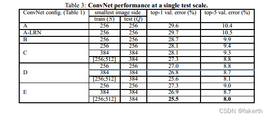
First, we note that using local response normalisation (A-LRN network) does not improve on the model A without any normalisation layers. We thus do not employ normalisation in the deeper architectures (B–E).

首先，我们注意到使用局部响应归一化（A-LRN网络）并不能提高不含任何归一化层的模型A的性能。因此，我们在更深的架构（B-E）中没有采用归一化。

Second, we observe that the classification error decreases with the increased ConvNet depth: from 11 layers in A to 19 layers in E. Notably, in spite of the same depth, the configuration C (which contains three 1 × 1 conv. layers), performs worse than the configuration D, which uses 3 × 3 conv. layers throughout the network. This indicates that while the additional non-linearity does help (C is better than B), it is also important to capture spatial context by using conv. filters with non-trivial receptive fields (D is better than C). The error rate of our architecture saturates when the depth reaches 19 layers, but even deeper models might be beneficial for larger datasets. We also compared the net B with a shallow net with five 5 × 5 conv. layers, which was derived from B by replacing each pair of 3 × 3 conv. layers with a single 5 × 5 conv. layer (which has the same receptive field as explained in Sect. 2.3). The top-1 error of the shallow net was measured to be 7% higher than that of B (on a center crop), which confirms that a deep net with small filters outperforms a shallow net with larger filters.

第二，我们观察到随着ConvNet深度的增加，分类误差逐渐减小：从A的11层到E的19层。值得注意的是，尽管深度相同，但包含三个1×1卷积层的配置C表现比使用整个网络的3×3卷积层的配置D更差。这表明，尽管额外的非线性确实有帮助（C优于B），但使用具有非平凡接受域的卷积滤波器来捕获空间上下文也很重要（D优于C）。我们的体系结构的错误率在深度达到19层时饱和，但对于更大的数据集，甚至更深的模型可能是有益的。我们还将net B与一个浅层的网络进行了比较，该网络具有五个5×5卷积层，是通过用一个单独的5×5卷积层替换每对3×3卷积层从B中派生出来的（如第2.3节所述具有相同的接受域）。浅层网络的top-1误差被测量为比B的高7％（在中心裁剪上），这证实了具有小滤波器的深度网络优于具有大滤波器的浅层网络。

Finally, scale jittering at training time (S ∈ [256; 512]) leads to significantly better results than training on images with fixed smallest side (S = 256 or S = 384), even though a single scale is used at test time. This confirms that training set augmentation by scale jittering is indeed helpful for capturing multi-scale image statistics.

最后，训练时的尺度抖动（S ∈ [256，512]）相对于在固定的最小边上训练（S = 256或S = 384）可以显着提高结果，尽管测试时仅使用单个尺度。这证实了通过尺度抖动进行训练集扩充确实有助于捕获多尺度图像统计信息。

4.2 MULTI-SCALE EVALUATION

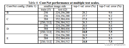
Having evaluated the ConvNet models at a single scale, we now assess the effect of scale jittering at test time. It consists of running a model over several rescaled versions of a test image (corresponding to different values of Q), followed by averaging the resulting class posteriors. Considering that a large discrepancy between training and testing scales leads to a drop in performance, the models trained with fixed S were evaluated over three test image sizes, close to the training one: Q = {S − 32, S, S + 32}. At the same time, scale jittering at training time allows the network to be applied to a wider range of scales at test time, so the model trained with variable S ∈ [Smin; Smax] was evaluated over a larger range of sizes Q = {Smin, 0.5(Smin + Smax), Smax}.

在评估了单一尺度下的ConvNet模型后，我们现在评估了测试时尺度扰动的影响。它包括在测试图像的几个重新缩放版本上运行模型(对应不同的Q值)，然后平均得出结果的类后验概率。考虑到训练和测试尺度之间的巨大差异会导致性能下降，因此使用固定S训练的模型在三个接近训练尺度的测试图像尺寸上进行了评估：Q = {S-32，S，S + 32}。同时，训练时的尺度扰动允许网络在测试时应用于更广泛的尺度范围，因此使用可变S∈[Smin；Smax]训练的模型在更大的尺寸范围Q = {Smin，0.5(Smin + Smax)，Smax}上进行了评估。

The results, presented in Table 4, indicate that scale jittering at test time leads to better performance (as compared to evaluating the same model at a single scale, shown in Table 3). As before, the deepest configurations (D and E) perform the best, and scale jittering is better than training with a fixed smallest side S. Our best single-network performance on the validation set is 24.8%/7.5% top-1/top-5 error (highlighted in bold in Table 4). On the test set, the configuration E achieves 7.3% top-5 error.

在表格4中呈现的结果表明，测试时进行尺度抖动会导致更好的性能（相比在单个尺度上评估相同的模型，在表格3中展示）。与之前相同，最深层的配置（D和E）表现最佳，并且尺度抖动比使用固定最小边S进行训练效果更好。我们在验证集上的最佳单网络性能是24.8％/7.5％的top-1/top-5错误率（在表4中以粗体突出显示）。在测试集上，配置E实现了7.3％的top-5错误率。

在这里插入图片描述

4.3 MULTI-CROP EVALUATION

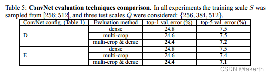
In Table 5 we compare dense ConvNet evaluation with mult-crop evaluation (see Sect. 3.2 for details). We also assess the complementarity of the two evaluation techniques by averaging their softmax outputs. As can be seen, using multiple crops performs slightly better than dense evaluation, and the two approaches are indeed complementary, as their combination outperforms each of them.As noted above, we hypothesize that this is due to a different treatment of convolution boundary conditions.

在表5中，我们比较了密集 ConvNet 评估和多裁剪评估(详见第3.2节)。我们还通过平均它们的softmax输出来评估两种评估技术的互补性。如表所示，使用多个裁剪的性能略优于密集评估，而且两种方法确实是互补的，它们的组合优于它们中的任何一种。如上所述，我们假设这是由于卷积边界条件的不同处理方式所导致的。

在这里插入图片描述

4.4 CONVNET FUSION

Up until now, we evaluated the performance of individual ConvNet models. In this part of the experiments, we combine the outputs of several models by averaging their soft-max class posteriors. This improves the performance due to complementarity of the models, and was used in the top ILSVRC submissions in 2012 (Krizhevsky et al, 2012) and 2013 (Zeiler & Fergus, 2013; Sermanet et al, 2014)

直到现在，我们一直在评估单个ConvNet模型的性能。在这部分实验中，我们通过平均其软最大类后验概率来结合几个模型的输出。由于模型的互补性，这种方法可以提高性能，并且在2012年（Krizhevsky等人，2012）和2013年（Zeiler＆Fergus，2013；Sermanet等人，2014）的ILSVRC比赛中被用于最高提交。

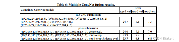
The results are shown in Table 6. By the time of ILSVRC submission we had only trained the single-scale networks, as well as a multi-scale model D (by fine-tuning only the fully-connected layers rather than all layers). The resulting ensemble of 7 networks has 7.3% ILSVRC test error.After the submission, we considered an ensemble of only two best-performing multi-scale models (configurations D and E), which reduced the test error to 7.0% using dense evaluation and 6.8% using combined dense and multi-crop evaluation. For reference, our best-performing single model achieves 7.1% error (model E, Table 5).

在表6中展示了结果。在提交ILSVRC比赛的时候，我们只训练了单尺度网络以及一个多尺度模型D(只微调全连接层而不是所有层)。由7个网络组成的集成模型的ILSVRC测试误差为7.3%。提交后，我们考虑了一个只包含最佳表现的两个多尺度模型(配置D和E)的集成模型，使用密集评估的测试误差降至7.0%，使用联合密集评估和多裁剪评估降至6.8%。作为参考，我们最佳的单一模型达到了7.1%的误差率（表5，模型E）。

在这里插入图片描述

4.5 COMPARISON WITH THE STATE OF THE ART

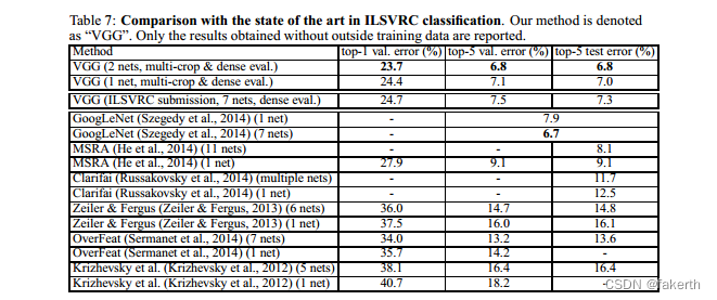
Finally, we compare our results with the state of the art in Table 7. In the classification task of ILSVRC-2014 challenge (Russakovsky et al, 2014), our “VGG” team secured the 2nd place with 7.3% test error using an ensemble of 7 models. After the submission, we decreased the error rate to 6.8% using an ensemble of 2 models.

最后，我们在表7中将我们的结果与现有技术水平进行比较。在ILSVRC-2014挑战赛的分类任务中（Russakovsky等人，2014），我们的“VGG”团队使用7个模型的集合获得了第二名，测试误差为7.3%。提交后，我们使用2个模型的集合将误差率降低到了6.8%。

As can be seen from Table 7, our very deep ConvNets significantly outperform the previous generation of models, which achieved the best results in the ILSVRC-2012 and ILSVRC-2013 competitions. Our result is also competitive with respect to the classification task winner (GoogLeNet with 6.7% error) and substantially outperforms the ILSVRC-2013 winning submission Clarifai, which achieved 11.2% with outside training data and 11.7% without it. This is remarkable, considering that our best result is achieved by combining just two models – significantly less than used in most ILSVRC submissions. In terms of the single-net performance, our architecture achieves the best result (7.0% test error), outperforming a single GoogLeNet by 0.9%. Notably, we did not depart from the classical ConvNet architecture of LeCun et al (1989), but improved it by substantially increasing the depth.

从表7中可以看出，我们的超深度卷积神经网络显着优于先前的模型代表，在ILSVRC-2012和ILSVRC-2013比赛中取得了最佳成绩。我们的结果也与分类任务优胜者（6.7％错误的GoogLeNet）具有竞争力，并且在性能上远远优于在ILSVRC-2013中获胜的Clarifai提交，后者通过使用外部训练数据达到11.2％的错误率，没有使用外部数据则为11.7％。值得注意的是，考虑到我们只使用了两个模型，我们的最佳结果非常优秀，比大多数ILSVRC提交的模型要少得多。就单个网络的性能而言，我们的架构取得了最佳结果（7.0％的测试误差），优于单个GoogLeNet 0.9％。值得注意的是，我们没有远离LeCun等人（1989）的经典ConvNet架构，而是通过大幅增加深度来改进它。

在这里插入图片描述

CONCLUSION

In this work we evaluated very deep convolutional networks (up to 19 weight layers) for largescale image classification. It was demonstrated that the representation depth is beneficial for the classification accuracy, and that state-of-the-art performance on the ImageNet challenge dataset can be achieved using a conventional ConvNet architecture (LeCun et al, 1989; Krizhevsky et al, 2012) with substantially increased depth. In the appendix, we also show that our models generalise well to a wide range of tasks and datasets, matching or outperforming more complex recognition pipelines built around less deep image representations. Our results yet again confirm the importance of depth in visual representations

本研究中，我们评估了用于大规模图像分类的非常深的卷积神经网络（达到19个权重层）。研究表明，表示深度对分类准确性有益，并且可以使用传统的ConvNet架构（LeCun等人，1989; Krizhevsky等人，2012）实现ImageNet挑战数据集的最先进性能，但深度要大幅增加。在附录中，我们还展示了我们的模型可以很好地推广到各种任务和数据集，与建立在不那么深的图像表示周围的更复杂的识别管道相匹配或优于它们。我们的结果再次确认了视觉表示中深度的重要性。

ACKNOWLEDGEMENTS

这项工作是由ERC资助VisRec no。228180. 我们非常感谢NVIDIA公司捐赠用于本研究的图形处理器