【已解决】TD算法超详细解释和实现（Sarsa，n-step Sarsa，Q-learning）一篇文章看透彻！

郑重声明：本系列内容来源 赵世钰(Shiyu Zhao)教授的强化学习数学原理系列，本推文出于非商业目的分享个人学习笔记和心得。如有侵权，将删除帖子。原文链接：https://github.com/MathFoundationRL/Book-Mathmatical-Foundation-of-Reinforcement-Learning

上一节我们讲到，Robbins-Monro Algorithm算法解决了下面的这个求期望的问题，本节我们把问题稍微复杂化一点。

看下边这个期望的计算：

假设我们可以获得随机变量$R,X$的样本那么可以定义下面的函数：

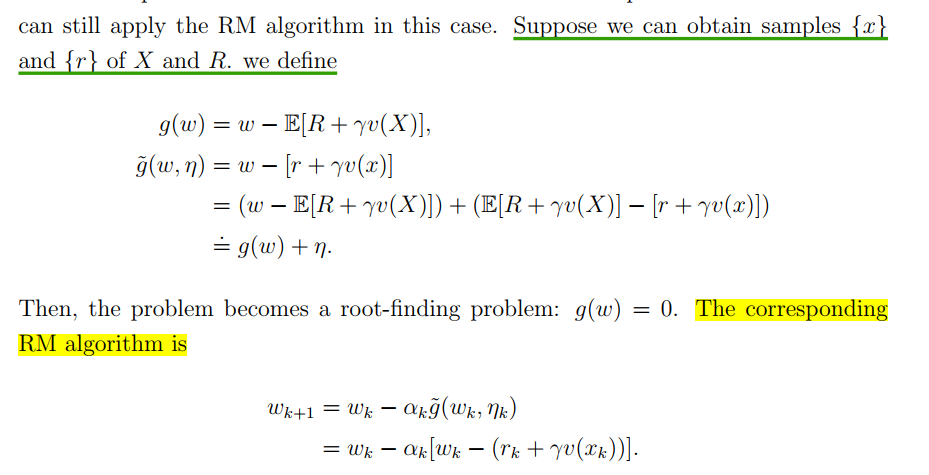
其实，也就是是把之前的一个随机变量变成了一个多元随机变量的函数。下面我们展示，这个例子其实和TD算法的表达很相似了。

TD learning of state values

本节所指的TD算法特指用于估测状态价值的经典TD算法。

算法

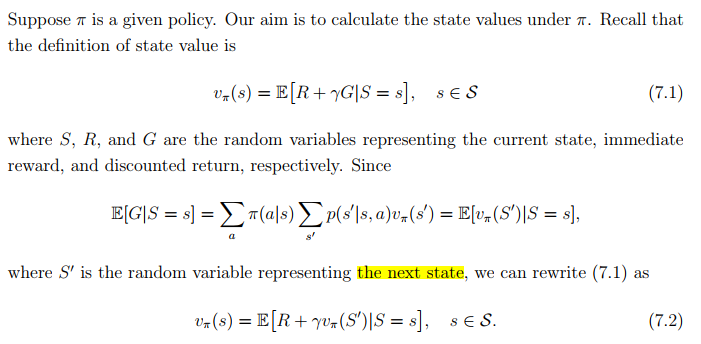
这个状态价值的期望形式的表示，有时候被称为贝尔曼期望等式，其实是贝尔曼方程的另一种表达，它是设计和分析TD算法的重要工具。那怎么去解这个方程呢？这就用到了我们前面小节讲到的，RM算法以及随机梯度下降的思想。这里需要注意，每次更新是一次更新一个状态的价值。

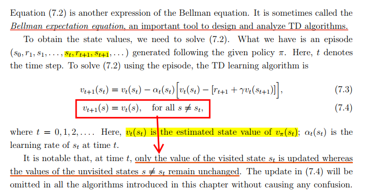
推导

通过应用RM算法求解贝尔曼方程，我们可以导出TD算法。

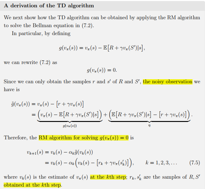
在了解了RM算法的前提下，上面的算法并不难理解。另外，RM算法关于状态价值的解，7.5式，有两个假设值得考虑：

显然，假设1)和2)在实践中都无法实现，对于1）是因为实践中的数据都是一个个的episodes，s在其中只是被抽样到的一个，不能确保每一个episodes都是从s开始的；对于2）我们怎么可以在事先知道其他状态的价值呢，要知道每一个状态的价值都是被算法估测出来的。

如何在RM算法中去除这两个假设的约束呢？

也就是说，RM算法中用的数据以s为起点，把第k次抽样$s^{\prime }$ 得到的 $s_k^{\prime }$ 作为下一个状态，而这样并不能充分利用全局的状态来进行价值的估测，要知道我们得到的数据是一个个episodes，每次只用episodes的开头部分的数据是不可行的。

下面这个地方说明了k和t 的不同：

所以，我们修改了算法使用的序列样本数据的形式为： { ( s t , r t + 1 , s t + 1 ) } \left\{\left(s_t, r_{t+1}, s_{t+1}\right)\right\} {(st​,rt+1​,st+1​)}

另一个关于状态价值的改动就不必说了，因为算法更新过程中的状态价值并不是策略的状态价值函数，一个是进行时态，一个是完成时态。

性质

首先，我们要深入分析一下TD算法的表达式：

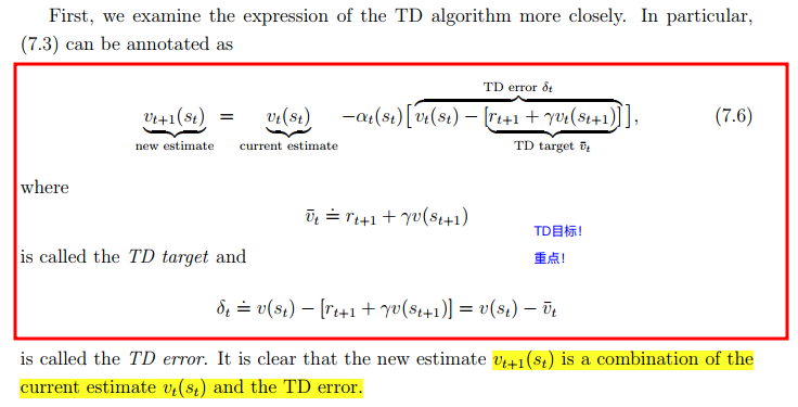
第二，TD算法也有局限性，它只能估测状态的价值，为了找到最优的策略，我们还需要进一步计算动作价值，然后做策略改进。（当然啦，在系统模型不可知的时候，我们可以直接去估测动作价值）

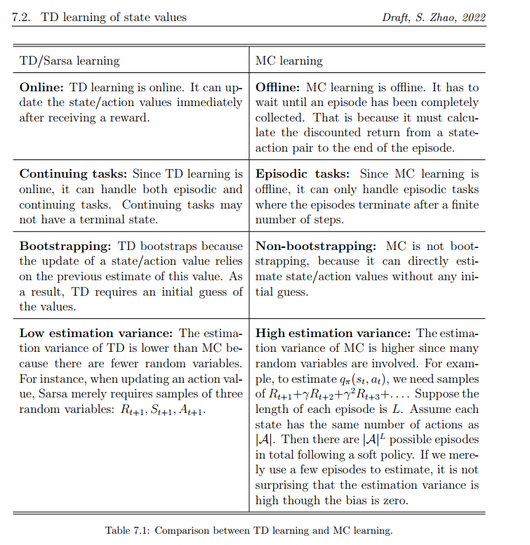
第三，TD算法和MC算法都是无模型的，TD算法和MC相比的优势和劣势是什么呢？我们可以从下表看到：

（PS，个人觉得这个表意义重大，值得反复观看！）

1. 区分了online learning 和offline learning
2. 区分了持续性任务和周期性任务
3. 区分了自举和非自举
4. 分析了MC和TD算法的方差比较和成因，赵世钰老师牛逼！

收敛性分析

略了

TD learning of action values: Sarsa

算法

sarsa算法的作用是去估计动作的价值。

在第t步，只有当前的状态-动作对被更新。

1. SARSA的名字来源？

   1. Sarsa is the abbreviation of state-action-reward-state-action.

2. SARSA 和 TD的关系？

   1. We can obtain Sarsa by replacing the state value estimate v(s) in the TD algorithm with the action value estimate q(s,a). As a result, Sarsa is nothing but an action-value version of the TD algorithm.

3. Sarsa is a stochastic approximation algorithm solving the following equation:

   1. 

4. SARSA算法是贝尔曼方程的状态-动作价值形式。

5. SARSA算法的收敛性对学习率 $\alpha$ 有要求：

实现

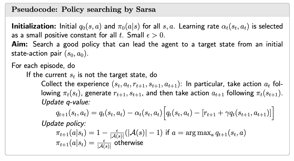
先捋一下思路，RL算法的目的是找最优的策略。而SARSA算法目前只能求解最优的状态-动作价值。收基于模型的策略迭代算法的启发，我们可以把策略迭代引入SARSA，分成两步来找最优策略：The first is to update the q-value of the visited state-action pair. The second is to update the policy as an ε-greedy one.有两点值得注意：

第一点：之前值迭代和一些基于模型的策略迭代在每一次迭代之后是更新了所有的状态的价值的，而SARSA在每一步，仅仅更新一个状态-动作对的价值，然后！立马！状态$s_t$的策略就被随之更新。尽管啊，这样的更新策略可能是不够精确的。

第二点： policy 更新过程是 ε-greedy 的，从而保证所有的状态-动作对都被访问到。

我们来看一个例子，无图无真相！

实验设定如下：

下图显示的是SARSA最终算出来的策略，注意，this policy can successfully reach the target state from the starting state. However, the policies for other states may not be optimal. That is because the other states are not of interest and every episode ends when the target state is reached. If we need to find the optimal policies for all states, we should ensure all the states are visited sufficiently many times by, for example, starting episodes from different states. （说白了，就是初始的那个状态唯我独尊，但是对其他状态作为初始状态的情况，这个生成的策略并不是最优的。要想对所有状态找最优策略，那么我们需要把每一个状态作为开始状态，得到充分多的状态动作对作为episods训练数据。）

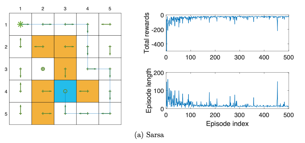
右上图可以看到，每一个episode的sum reward在逐渐增高。从右下图可以看到，episodes的长度在逐渐变短。

TD learning of action values: Expected Sarsa

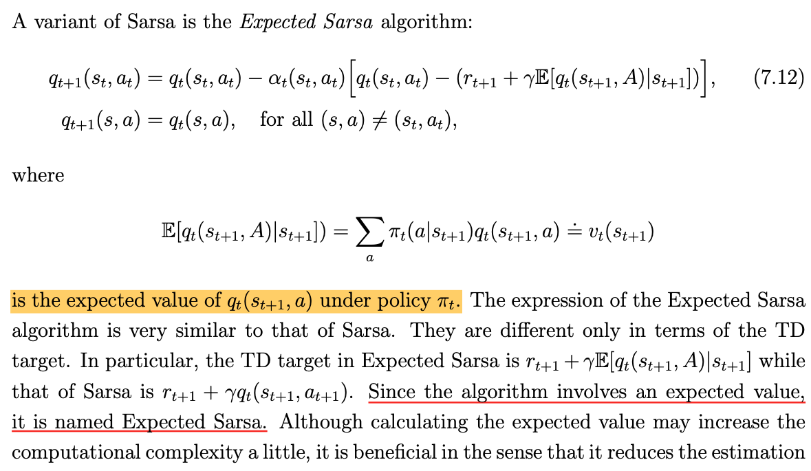
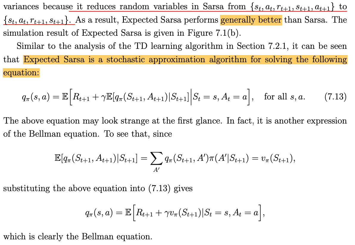
原理

实现

在算法实现上面，除了q-value的更新过程不一样之外，其他的和SARSA差不多。

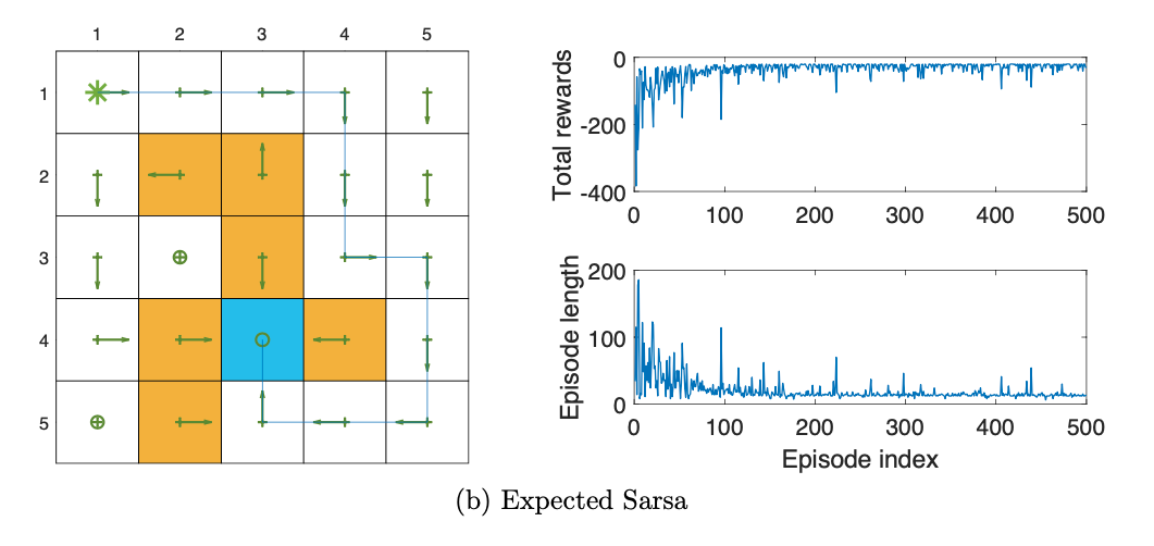
实验

TD learning of action values: n-step Sarsa

和Sarsa的区别主要是discounted return项的展开的长度（the different decomposition structure ）的不一样：

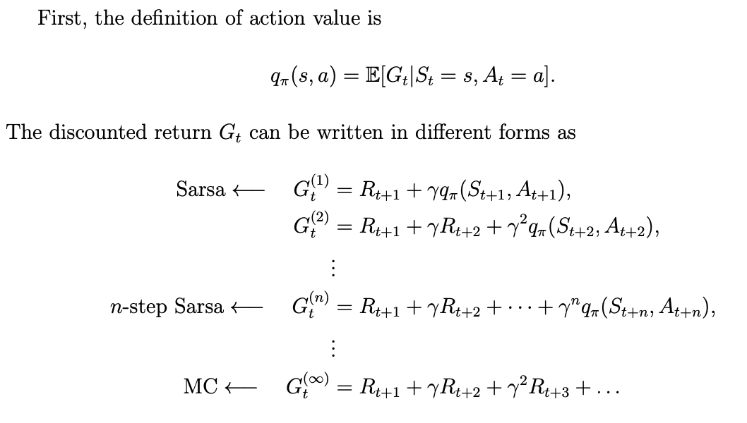
实现

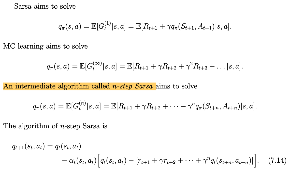
注意要点：

However, we can wait until time t + n to update the q-value of (St,At). To that end, (7.14) can be modified to

区别就是，我们通过等待n步再计算q值，从而让它更准确一点。

总结

1. Specifically, if n is selected to be a large number, its performance is close to MC learning and hence has a large variance but a small bias. If n is selected to be small, its performance is close to Sarsa and hence has a relatively large bias due to the initial guess and relatively low variance.
2. Finally, n-step Sarsa is also for policy evaluation. It can be combined with the policy improvement step to search for optimal policies.

TD learning of optimal action values: Q-learning 放大招！

SARSA只能是估测每个状态动作价值，必须要借助策略迭代方法来求最优状态动作价值，而By contrast, Q-learning can directly estimate optimal action values.

算法

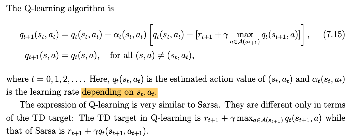
Q: Q-learning的更新过程需要的数据是什么呢？

A：反正不需要$a_{t+1}$

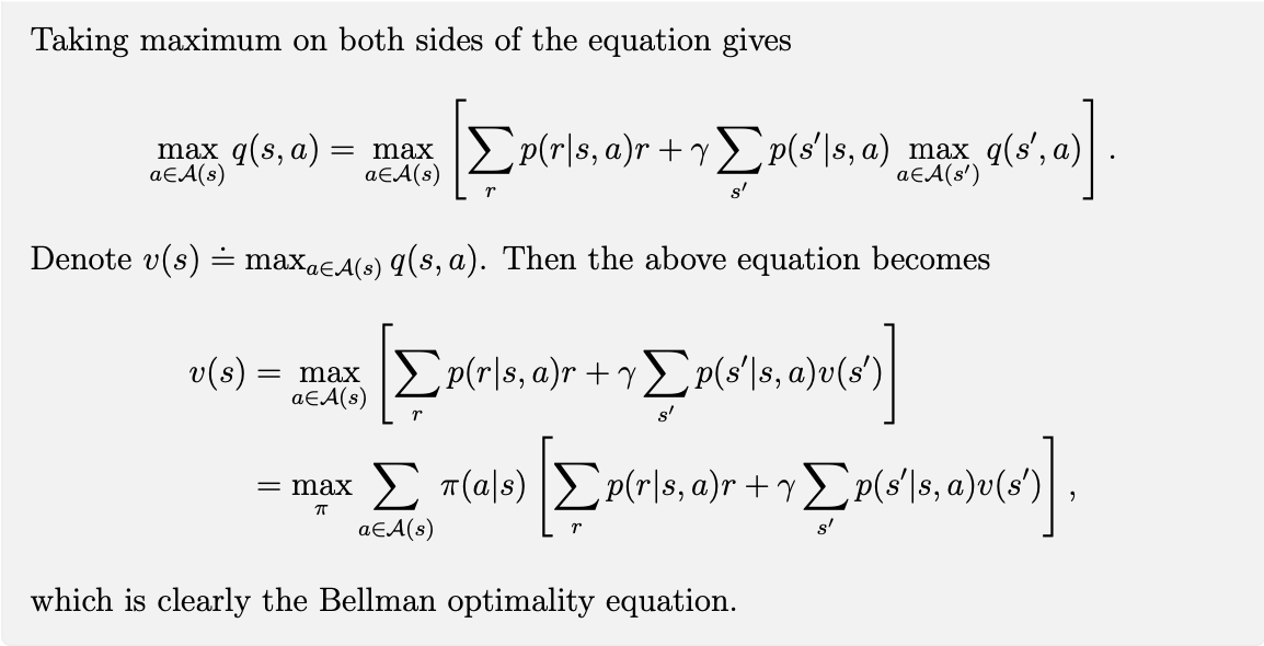
Q-learning其实是在使用随机估测方法在计算下面的方程：

很简单可以证明这个方程其实就是贝尔曼最优方程：

展开上式得到：

实现

虽然Q-learning 是off-policy（这是由算法本身决定的），但是它可以Work online 或者 offline，这是和实现有关系的。

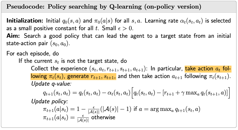
The on-policy version is the same as Sarsa except for the TD target in the q-value update step. In this case, the behavior policy is the same as the target policy, which is an ε-greedy policy.

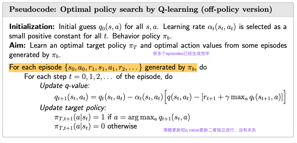
In the off-policy version, the episode is generated by the behavior policy πb which can be any policy. If we would like to sample experiences for every state-action pair, πb should be selected to be exploratory.（意思是把学习率设置得比较大）

Here, the target policy πT is greedy rather than ε-greedy. That is because the target policy is not used to generate episodes and hence is not required to be exploratory.

Moreover, the off-policy version of Q-learning presented here is offline. That is because all the experience samples are collected first and then processed to estimate an optimal target policy. Of course, it can be modified to become online. Once a sample is collected, the sample can be used to update the q-value and target policy immediately. Nevertheless, the updated target policy is not used to generate new samples. （online版本的Q-learning，没有使用更新后的策略去生成样本进行迭代，否则的话就是on-policy了）

例子（图示）

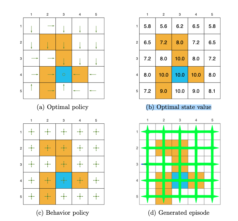
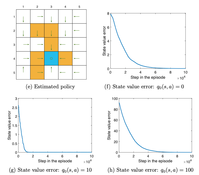
Figure 7.2: Examples to demonstrate off-policy learning by Q-learning. The optimal policy and optimal state values are shown in (a) and (b), respectively. The behavior policy and the generated single episode are shown in © and (d), respectively. The estimated policy and the estimation error evolution are shown in (e) and (f), respectively. The cases with different initial q-value are shown in (g) and (h), respectively.

由于最优策略有多个，所以Q-learning学到的e和原始的最优策略设定b并不一样。

由于Q-learning的自举特性，初始状态价值的设定和收敛的速度是息息相关的。（g）和（h）的区别就可以看出来。

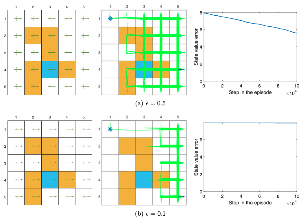
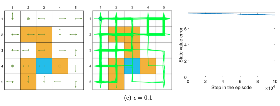
Figure 7.3: Performance of Q-learning given different non-exploratory behavior policies. The figures in the left column show the behavior policies. The figures in the middle column show the generated episodes following the corresponding behavior policies. The episode in every example has 100,000 steps. The figures in the right column show the evolution of the root-mean-squared error of the estimated state values, which are calculated from the estimated action values.（上面这些图，中间的那列是基于右边的策略生成的轨迹。

可以看出啊，当行为策略不是探索的时候，（在7.3中是固定的），学习的效果变得很差。比如，状态值的误差对 $ϵ$的缩小很敏感。

A unified viewpoint

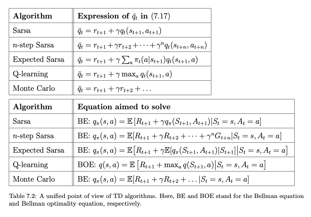
It is worth mentioning that there are some methods to convert an on-policy learning algorithm to off-policy. Importance sampling is a widely used method¹.

Moreover, there are various extensions of the TD algorithms introduced in this chapter. For example, the TD(λ) method provides a more general and unified framework for TD learning. The TD algorithm in Section 7.6 is simply TD(0), a special case of TD(λ). Details of TD(λ) can be found in ².

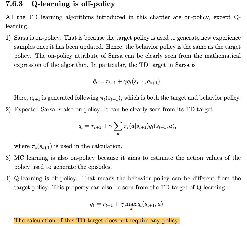
注意：Q-learning is off-policy！！！

答疑环节

1. 时间差分TD这个词在TD learning中是什么意思？

   1. Every TD algorithm has a TD error, which represents the deficiency between the new sample and the current estimates. This deficiency is between two different time steps and hence called temporal difference.

2. TD learning 算法只是在估计动作的价值，它怎么可以用来找寻最优策略呢？

   1. To obtain an optimal policy, the value estimation process should interact with the policy update process. That is, after a value is updated, the corresponding policy should be updated. Then, a new sample generated by the updated policy is used to update values again. This is the idea of generalized policy iteration.

3. TD learning 算法的收敛要求学习率逐渐收敛到0，为什么实践中学习率被设置为常量呢？

   1. The fundamental reason is the policy to be evaluated is nonstationary. A TD learning algorithm like Sarsa aims to estimate the action values of a given fixed policy. In other words, it aims to evaluate the given policy. If the policy is stationary, the learning rate can decrease to zero gradually to ensure convergence with probability 1 as stated in Theorem 7.1. （在策略评估场景下，我们假定策略不变
   2. However, when we put Sarsa in the context of optimal policy searching, the value estimation process keeps interacting with the policy update process. Therefore, the policy that Sarsa aims to evaluate keeps changing. In this case, we need to use a constant learning rate because, every time we have a new policy to evaluate, the learning rate cannot be too small. The drawback of a constant learning rate is that the value estimate may still fluctuate eventually. However, as long as the constant learning rate is sufficiently small, the fluctuation would not jeopardize the convergence.（在最优策略寻找场景下，策略在不断地更新，面对新的策略，我们不能让学习率太小了。缺点呢，就是状态价值的估计值会一直震荡。这个情况可以通过把学习率设置得比较小来实现。

4. Should we estimate the optimal policies for all states or a subset of states?

5. It depends on the task. One may have noticed that some tasks in the illustrative examples in this chapter are not to find the optimal policies for all states. Instead, they only need to find a good path from a specific starting state to the target state. Such a task is not data demanding because we do not need to visit every state-action pair sufficiently many times. As shown in the examples in Figure 7.1, even if some states are not visited, we can still obtain a good path.

6. It, however, must be noted that the path is only good but not guaranteed to be optimal. That is because not all state-action pairs have been explored and there may be better paths unexplored. Nevertheless, given sufficient data, there is a high probability for us to find a good or locally optimal path. By locally optimal, we mean the path is optimal within a neighborhood of the path.（重点理解一下，locally optimal这个概念！

7. 为啥 Q-learning是off-policy的，而别的TD算法都是 on-policy的，而根本的原因是什么！

   • Q-learning aims to solve the Bellman optimality equation. The other TD algorithms are on-policy because they aim to solve the Bellman equation of a given policy.
   • Since the Bellman optimality equation does not depend on any specific policy, it can use the experience samples generated by any other policies to estimate the optimal policy. However, the Bellman equation depends on a given policy, solving it of course requires the experience samples generated by the given policy. （看明白了，背后的原因是Bellman optimality equation 和 Bellman equation 在数学形式上的差别！！

---

---

1. T. C. Hesterberg, Advances in importance sampling. PhD Thesis, Stanford Univer- sity, 1988. ↩︎

2. R. S. Sutton, “Learning to predict by the methods of temporal differences,” Machine Learning, vol. 3, no. 1, pp. 9–44, 1988. ↩︎