需要源码请点赞关注收藏后评论区留下QQ~~~
一、策略梯度法
策略梯度法(PG)利用策略函数来选择动作,同时使用值函数来辅助策略函数参数的更新,根据策略类型的不同,可以分为随机策略梯度和确定性策略梯度
策略梯度法与值函数逼近法相比优点如下
1:平滑收敛
在学习过程中,PG法每次更新策略函数,权重参数都会朝着最优值变化,且只发生微小变化,有很强的收敛性,值函数逼近法基于贪心策略对策略进行改进,有些价值函数在后期会一直围绕着最优价值函数持续小的震荡而不收敛 即出现策略退化
2:处理连续动作空间任务
PG法可以直接得到一个策略,而值函数逼近法需要对比状态S中的所有动作的价值
3:学习随机策略
PG法能够输出随机策略,而值函数逼近法基于贪心方法,每次输出的都是确定性函数
PG法缺点如下
1:PG法通常只能收敛到局部最优解
2:PG法的易收敛性和学习过程平滑优势,都是使Agent尝试过多的无效探索,从而造成学习效率低,整体策略方差偏大,以及存在累积错误带来的过高估计问题
二、蒙特卡洛策略梯度法(REINFORCE)
蒙特卡洛策略梯度法是一种针对情节式问题的,基于MC算法的PG法
REINFORCE算法采用MC算法来计算动作值函数,只考虑Agent在状态S下实际采取的动作,该方法可以从理论上保存策略参数的收敛性
1:实验环境设置
引入短走廊网格世界环境 如下图
每步的收益是-1,对于三个非终止状态都有两个动作可以选择,向左或者向右,特殊的是,第一个状态向左走会保持原地不动,而在第二个状态执行的动作会导致向相反的方向移动
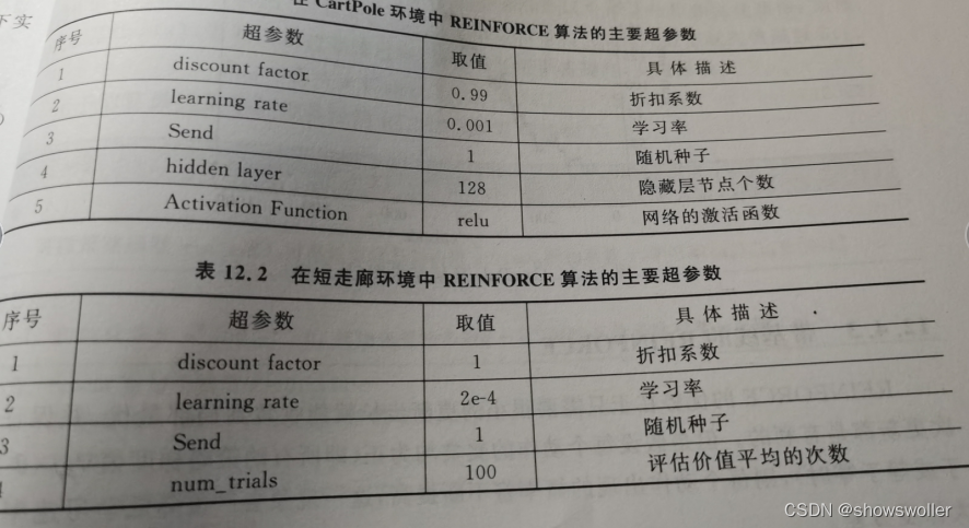
部分超参数列表如下
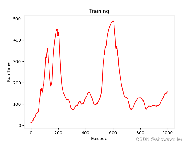
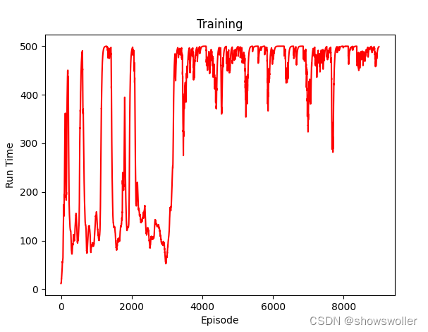
2:实验结果分析
每个环境下算法的训练情节数均为1000个情节,这是因为两个环境在1000个情节后都能收敛,如下图所示REINFORCE算法在短走廊环境和CartPole环境的效果整体上都呈现稳步上升,后平稳的学习趋势
迭代一千次后如下 (每隔一千次输出一次可视化图像)
迭代两千次后效果如下


迭代8000次后如下 发现基本已经在高位收敛
三、代码
部分源码如下
# 代38-REINFORCE算法的实验过程


#CartPole环境
import argparse
import gym
import numpy as np
from itertools import count

import torch
import torch.nn as nn
import torch.nn.functional as F
import torch.optim as optim
from torch.distributions import Categorical
import matplotlib.pyplot as plt

import os
os.environ["KMP_DUPLICATE_LIB_OK"]="TRUE"

parser = argparse.ArgumentParser(description='PyTorch REINFORCE example')
parser.add_argument('--gamma', type=float, default=0.99, metavar='G',
                    help='discount factor (default: 0.99)')
parser.add_argument('--seed', type=int, default=543, metavar='N',
                    help='random seed (default: 543)')
parser.add_argument('--render', action='store_true',
                    help='render the environment')
parser.add_argument('--log-interval', type=int, default=10, metavar='N',
                    help='interval between training status logs (default: 10)')
args = parser.parse_args()


env = gym.make('CartPole-v1')
env.seed(args.seed)
torch.manual_seed(args.seed)


class Policy(nn.Module):
    def __init__(self):
        super(Policy, self).__init__()
        self.affine1 = nn.Linear(4, 128)
        self.dropout = nn.Dropout(p=0.6)
        self.affine2 = nn.Linear(128, 2)

        self.saved_log_probs = []
        self.rewards = []

    def forward(self, x):
        x = self.affine1(x)
        x = self.dropout(x)
        x = F.relu(x)
        action_scores = self.affine2(x)
        return F.softmax(action_scores, dim=1)


policy = Policy()
optimizer = optim.Adam(policy.parameters(), lr=1e-2)
eps = np.finfo(np.float32).eps.item()


def select_action(state):
    state = torch.from_numpy(state).float().unsqueeze(0)
    probs = policy(state)
    m = Categorical(probs)
    action = m.sample()
    policy.saved_log_probs.append(m.log_prob(action))
    return action.item()


def finish_episode():
    R = 0
    policy_loss = []
    rewards = []
    for r in policy.rewards[::-1]:
        R = r + args.gamma * R
        rewards.insert(0, R)
    rewards = torch.tensor(rewards)
    rewards = (rewards - rewards.mean()) / (rewards.std() + eps)
    for log_prob, reward in zip(policy.saved_log_probs, rewards):
        policy_loss.append(-log_prob * reward)
    optimizer.zero_grad()
    policy_loss = torch.cat(policy_loss).sum()
    policy_loss.backward()
    optimizer.step()
    del policy.rewards[:]
    del policy.saved_log_probs[:]

def plot(epi, run_time):

    plt.title('Training')
    plt.xlabel('Episode')
    plt.ylabel('Run Time')
    plt.plot(epi, run_time, color='red')
    plt.show()

def main():
    running_reward = 10
    running_rewards = []
    i_episodes = []
    for i_episode in range(10000):
        state, ep_reward = env.reset(), 0
        for t in range(1, 10000):  # Don't infinite loop while learning
            action = select_action(state)
            state, reward, done, _ = env.step(action)
            if args.render:
                env.render()
            policy.rewards.append(reward)
            ep_reward += reward
            if done:
                break

        running_reward = 0.05 * ep_reward + (1 - 0.05) * running_reward
        finish_episode()
        running_rewards.append(running_reward)
        i_episodes.append(i_episode)
        if i_episode % args.log_interval == 0:

            print('Episode {}\tLast length: {:2f}\tAverage length: {:.2f}'.format(
                i_episode, ep_reward, running_reward))
        if (i_episode % 1000 == 0):
            plot(i_episodes, running_rewards)
    np.save(f"putu", running_rewards)
if __name__ == '__main__':
    main()


# 短走廊环境
import numpy as np
import matplotlib
matplotlib.use('Agg')
import matplotlib.pyplot as plt
from tqdm import tqdm

def true_value(p):
    """ True value of the first state
    Args:
        p (float): probability of the action 'right'.
    Returns:
        True value of the first state.
        The expression is obtained by manually solving the easy linear system
        of Bellman equations using known dynamics.
    """
    return (2 * p - 4) / (p * (1 - p))

class ShortCorridor:
    """
    Short corridor environment, see Example 13.1
    """
    def __init__(self):
        self.reset()

    def reset(self):
        self.state = 0

    def step(self, go_right):
        """
        Args:
            go_right (bool): chosen action
        Returns:
            tuple of (reward, episode terminated?)
        """
        if self.state == 0 or self.state == 2:
            if go_right:
                self.state += 1
            else:
                self.state = max(0, self.state - 1)
        else:
            if go_right:
                self.state -= 1
            else:
                self.state += 1

        if self.state == 3:
            # terminal state
            return 0, True
        else:
            return -1, False

def softmax(x):
    t = np.exp(x - np.max(x))
    return t / np.sum(t)

class ReinforceAgent:
    """
    ReinforceAgent that follows algorithm
    'REINFORNCE Monte-Carlo Policy-Gradient Control (episodic)'
    """
    def __init__(self, alpha, gamma):
        # set values such that initial conditions correspond to left-epsilon greedy
        self.theta = np.array([-1.47, 1.47])
        self.alpha = alpha
        self.gamma = gamma
        # first column - left, second - right
        self.x = np.array([[0, 1],
                           [1, 0]])
        self.rewards = []
        self.actions = []

    def get_pi(self):
        h = np.dot(self.theta, self.x)
        t = np.exp(h - np.max(h))
        pmf = t / np.sum(t)
        # never become deterministic,
        # guarantees episode finish
        imin = np.argmin(pmf)
        epsilon = 0.05

        if pmf[imin] < epsilon:
            pmf[:] = 1 - epsilon
            pmf[imin] = epsilon

        return pmf

    def get_p_right(self):
        return self.get_pi()[1]

    def choose_action(self, reward):
        if reward is not None:
            self.rewards.append(reward)

        pmf = self.get_pi()
        go_right = np.random.uniform() <= pmf[1]
        self.actions.append(go_right)

        return go_right

    def episode_end(self, last_reward):
        self.rewards.append(last_reward)

        # learn theta
        G = np.zeros(len(self.rewards))
        G[-1] = self.rewards[-1]

        for i in range(2, len(G) + 1):
            G[-i] = self.gamma * G[-i + 1] + self.rewards[-i]

        gamma_pow = 1

        for i in range(len(G)):
            j = 1 if self.actions[i] else 0
            pmf = self.get_pi()
            grad_ln_pi = self.x[:, j] - np.dot(self.x, pmf)
            update = self.alpha * gamma_pow * G[i] * grad_ln_pi

            self.theta += update
            gamma_pow *= self.gamma

        self.rewards = []
        self.actions = []

class ReinforceBaselineAgent(ReinforceAgent):
    def __init__(self, alpha, gamma, alpha_w):
        super(ReinforceBaselineAgent, self).__init__(alpha, gamma)
        self.alpha_w = alpha_w
        self.w = 0

    def episode_end(self, last_reward):
        self.rewards.append(last_reward)

        # learn theta
        G = np.zeros(len(self.rewards))
        G[-1] = self.rewards[-1]

        for i in range(2, len(G) + 1):
            G[-i] = self.gamma * G[-i + 1] + self.rewards[-i]

        gamma_pow = 1

        for i in range(len(G)):
            self.w += self.alpha_w * gamma_pow * (G[i] - self.w)

            j = 1 if self.actions[i] else 0
            pmf = self.get_pi()
            grad_ln_pi = self.x[:, j] - np.dot(self.x, pmf)
            update = self.alpha * gamma_pow * (G[i] - self.w) * grad_ln_pi

            self.theta += update
            gamma_pow *= self.gamma

        self.rewards = []
        self.actions = []

def trial(num_episodes, agent_generator):
    env = ShortCorridor()
    agent = agent_generator()

    rewards = np.zeros(num_episodes)
    for episode_idx in range(num_episodes):
        rewards_sum = 0
        reward = None
        env.reset()

        while True:
            go_right = agent.choose_action(reward)
            reward, episode_end = env.step(go_right)
            rewards_sum += reward

            if episode_end:
                agent.episode_end(reward)
                break

        rewards[episode_idx] = rewards_sum

    return rewards

def example_13_1():
    epsilon = 0.05
    fig, ax = plt.subplots(1, 1)

    # Plot a graph
    p = np.linspace(0.01, 0.99, 100)
    y = true_value(p)
    ax.plot(p, y, color='red')

    # Find a maximum point, can also be done analytically by taking a derivative
    imax = np.argmax(y)
    pmax = p[imax]
    ymax = y[imax]
    ax.plot(pmax, ymax, color='green', marker="*", label="optimal point: f({0:.2f}) = {1:.2f}".format(pmax, ymax))

    # Plot points of two epsilon-greedy policies
    ax.plot(epsilon, true_value(epsilon), color='magenta', marker="o", label="epsilon-greedy left")
    ax.plot(1 - epsilon, true_value(1 - epsilon), color='blue', marker="o", label="epsilon-greedy right")

    ax.set_ylabel("Value of the first state")
    ax.set_xlabel("Probability of the action 'right'")
    ax.set_title("Short corridor with switched actions")
    ax.set_ylim(ymin=-105.0, ymax=5)
    ax.legend()

    plt.savefig('../images/example_13_1.png')
    plt.close()

def figure_13_1():
    num_trials = 100
    num_episodes = 1000
    gamma = 1
    agent_generators = [lambda : ReinforceAgent(alpha=2e-4, gamma=gamma),
                        lambda : ReinforceAgent(alpha=2e-5, gamma=gamma),
                        lambda : ReinforceAgent(alpha=2e-3, gamma=gamma)]
    labels = ['alpha = 2e-4',
              'alpha = 2e-5',
              'alpha = 2e-3']

    rewards = np.zeros((len(agent_generators), num_trials, num_episodes))

    for agent_index, agent_generator in enumerate(agent_generators):
        for i in tqdm(range(num_trials)):
            reward = trial(num_episodes, agent_generator)
            rewards[agent_index, i, :] = reward

    plt.plot(np.arange(num_episodes) + 1, -11.6 * np.ones(num_episodes), ls='dashed', color='red', label='-11.6')
    for i, label in enumerate(labels):
        plt.plot(np.arange(num_episodes) + 1, rewards[i].mean(axis=0), label=label)
    plt.ylabel('total reward on episode')
    plt.xlabel('episode')
    plt.legend(loc='lower right')

    plt.savefig('../images/figure_13_1.png')
    plt.close()

def figure_13_2():
    num_trials = 100
    num_episodes = 1000
    alpha = 2e-4
    gamma = 1
    ageninforce with baseline']

    rewards = np.zeros((len(agent_generators), num_trials, num_episodes))

    for agent_index, agent_generator in enumerate(agent_generators):
        for i in tqdm(range(num_trials)):
            reward = trial(num_episodes, agent_generator)
            rewards[agent_index, i, :] = reward

    plt.plot(np.arange(num_episodes) + 1, -11.6 * np.ones(num_episodes), ls='dashed', color='red', label='-11.6')
    for i, label in enumerate(labels):
        plt.plot(np.arange(num_episodes) + 1, rewards[i].mean(axis=0), label=label)
  _':
    example_13_1()
    figure_13_1()
    figure_13_2()
创作不易 觉得有帮助请点赞关注收藏~~~