来源：投稿 作者：175
编辑：学姐

往期内容：

从零实现深度学习框架1：RNN从理论到实战（理论篇）

从零实现深度学习框架2：RNN从理论到实战（实战篇）

从零实现深度学习框架3：再探多层双向RNN的实现（本篇）

在前面的文章中，我们实现了多层、双向RNN。但是这几天一直在思考，这种实现方式是不是有问题。因为RNN的实现关乎后面ELMo和seq2seq，所以不得不重视。

双向RNN的实现方式

以两层双向RNN为例。我们之前实现的方式类似如下图所示：

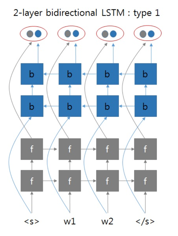
这两张图片来自于：https://github.com/pytorch/pytorch/issues/4930#issuecomment-361851298

就是正向RNN和反向RNN可以看成是两个独立的两层RNN网络，最终拼接了它们的输出。但是总感觉双向RNN不会这么简单，带着这个疑问去拜读了双向RNN的论文1，得到下面的这张图片：

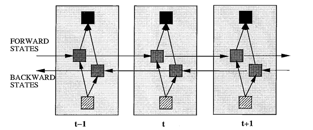
如果采用这种方式的话，那么两层双向RNN的实现应该像下图这样：

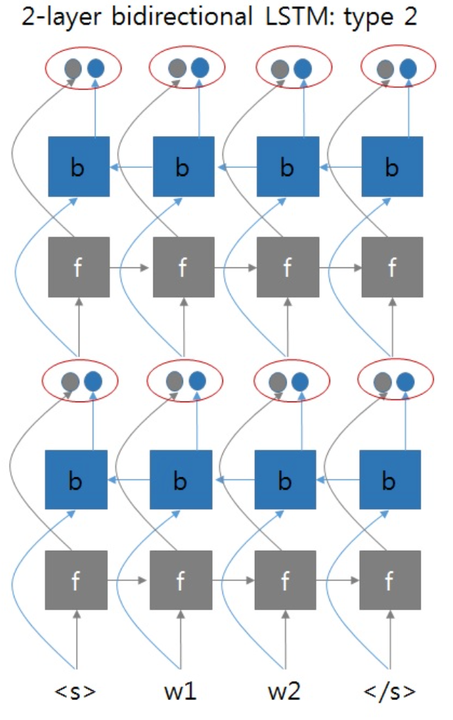
即第一层BRNN的输出同时考虑了正向和方向输出，将它们拼接在一起，作为第二层BRNN的输入。

但是这时遇到了一个问题，如果这样实现的话，那么输出的维度会怎样呢？BRNN中每层参数的维度会产生怎样的变化呢？

遇事不决找Torch，我们摸着PyTorch过河。

带着这个问题，我们去看PyTorch的文档，并查阅资料，梳理一下PyTorch实现的RNN(GRU、LSTM)中各种输入、输出、隐藏状态的维度。

理解RNN中的各种维度

以RNN为例，为什么不以最复杂的LSTM为例呢？因为LSTM参数过多，相比RNN太过复杂，不太容易理解。柿子要挑软的捏，我们理解了RNN，再去理解GRU或LSTM就会简单多了。

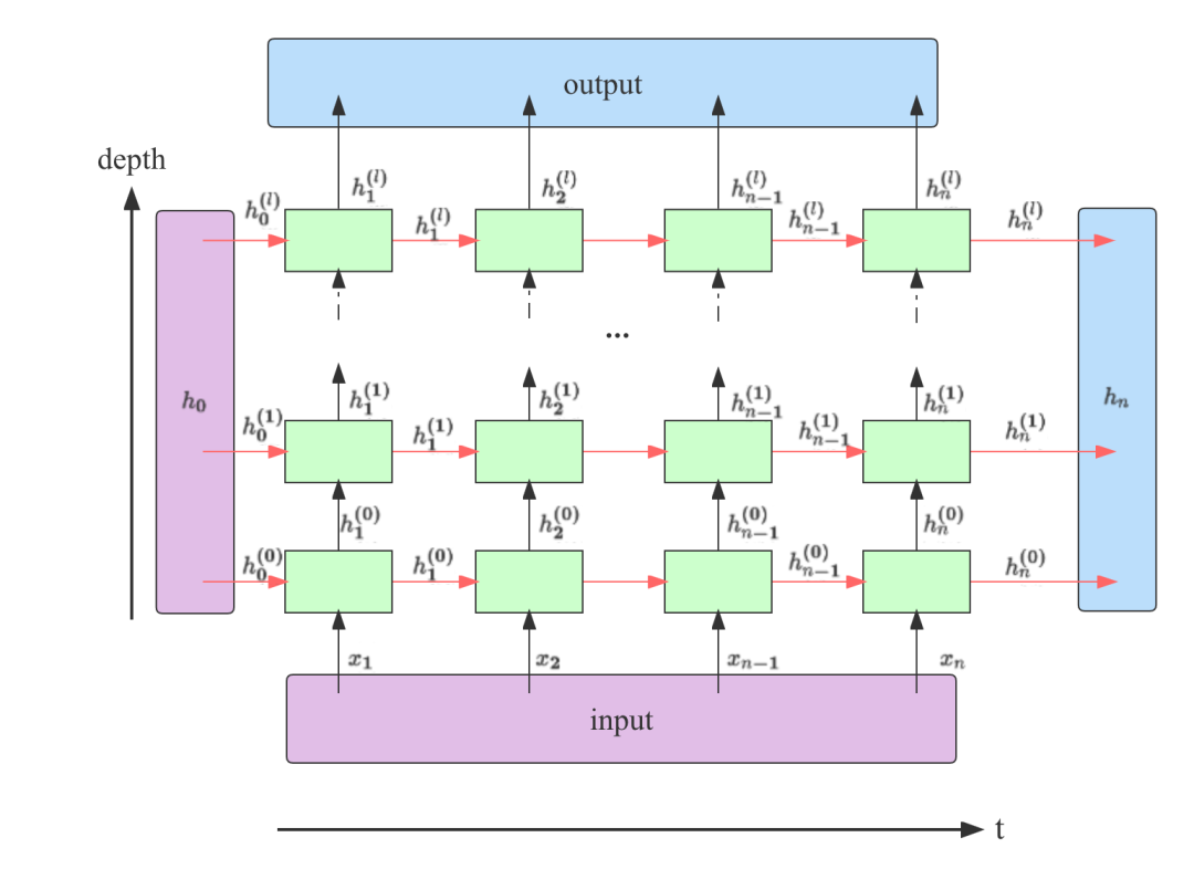
此图片参考了https://stackoverflow.com/a/48305882

从上图可以看出，在一个堆叠了l层的RNN中，output包含了最后一层RNN输出的所有隐藏状态；h_n包含了最后一个时间步上所有层的输出。

我们知道了它们的构成方式，下面看一下它们和上图中另外两个参数input和h_0在不同类型的RNN中维度如何2。

• inputRNN的输入序列。若batch_first=False，则其大小为(seq_len, batch_size, input_size)；若batch_first=True，则其大小为(batch_size, seq_len, input_size)；

• h_0 RNN的初始隐藏状态，可以为空。大小为(num_layers * num_directions, batch_size, hidden_size)；

• output RNN最后一层所有时间步的输出。若batch_first=False，则其大小为(seq_len, batch_size, num_directions * hidden_size)；若batch_first=True，则其大小为(batch_size, seq_len, num_directions * hidden_size)；

• h_nRNN中所有层最后一个时间步的隐藏状态。其大小为(num_layers * num_directions, batch_size, hidden_size)。不受batch_first的影响，其批次维度表现和batch_first=False一样。后面以代码实现的角度解释下为何这样，不代表官方的意图。

其中seq_len表示输入序列长度；batch_size表示批次大小；input_size表示输入的特征数量；num_layers表示层数；num_directions表示方向个数，单向RNN时为1，双向RNN时为2；hidden_size表示隐藏状态的特征数。

的形状应该和是一致的。

下面我们进行验证，首先看一下初始参数：

# 输入大小
INPUT_SIZE = 2
# 序列长度
SEQ_LENGTH = 5
# 隐藏大小
HIDDEN_SIZE = 3
# 批大小
BATCH_SIZE = 4

以及输入：

inputs = Tensor.randn(BATCH_SIZE, SEQ_LENGTH, INPUT_SIZE)

简单RNN

简单RNN就是单向单层RNN：

rnn = nn.RNN(input_size=INPUT_SIZE, hidden_size=HIDDEN_SIZE, num_layers=1, batch_first=True)

output, h_n = rnn(inputs)

print(f'Input Shape: {inputs.shape} ')
print(f'Output Shape: {output.shape} ')
print(f'Hidden Shape: {h_n.shape} ')

• inputs维度是我们预先定理好的，注意这里batch_first=True，所以inputs的第一个维度是批大小。

• output来自最后一层所有时间步的输出，时间步长度为5，包含整个批次内4条数据，每条数据的输出维度为3，可以理解为3分类问题。

• $h_n$来自单层最后一个时间步的隐藏状态，包含整个批次内4条数据，每条数据的输出维度为3。

Input Shape: (4, 5, 2) 
Output Shape: (4, 5, 3) 
Hidden Shape: (1, 4, 3) 

堆叠RNN

如果将层数改成3，我们就得到了3层RNN堆叠在一起的架构，来看下此时output和h_n的维度会发生怎样的变化。

rnn = nn.RNN(input_size=INPUT_SIZE, hidden_size=HIDDEN_SIZE, num_layers=3, batch_first=True)

output, h_n = rnn(inputs)

print(f'Input Shape: {inputs.shape} ')
print(f'Output Shape: {output.shape} ')
print(f'Hidden Shape: {h_n.shape} ')

Input Shape: (4, 5, 2) 
Output Shape: (4, 5, 3) 
Hidden Shape: (3, 4, 3) 

• output来自最后一层所有时间步的输出，时间步长度为5，包含整个批次内4条数据，每条数据的输出维度为3。其维度保持不变。

• h_n来自所有三层最后一个时间步的隐藏状态，包含整个批次内4条数据，每条数据的输出维度为3。可以看到，其输出的第一个维度大小由1变成了3，因为包含了3层的结果。

双向RNN

传入bidirectional=True，并将层数改回单层。

rnn = nn.RNN(input_size=INPUT_SIZE, hidden_size=HIDDEN_SIZE, num_layers=1, batch_first=True, bidirectional=True)

output, h_n = rnn(inputs)

print(f'Input Shape: {inputs.shape} ')
print(f'Output Shape: {output.shape} ')
print(f'Hidden Shape: {h_n.shape} ')

Input Shape: (4, 5, 2) 
Output Shape: (4, 5, 6) 
Hidden Shape: (2, 4, 3) 

• output来自最后一层所有时间步的输出，时间步长度为5，包含整个批次内4条数据，每条数据的输出维度为3，由于是双向，包含了两个方向上的结果，在此维度上进行堆叠，所以由3变成了6。

• h_n最后一个时间步的隐藏状态，包含整个批次内4条数据，每条数据的输出维度为3。第一个维度由1变成了2，因为在此维度上堆叠了双向的结果。

它们都包含了双向的结果，那如果想分别得到每个方向上的结果，要怎么做呢？

对于output。若batch_first=True，将output按照out.reshape(shape=(batch_size, seq_len, num_directions, hidden_size))进行变形，正向和反向的维度值为别为0和1。

对于h_n，按照h_n.reshape(shape=(num_layers, num_directions, batch_size, hidden_size))，正向和反向的维度值为别为0和1。

我们来对output进行拆分：

# batch_first=True
output_reshaped = output.reshape((BATCH_SIZE, SEQ_LENGTH, 2, HIDDEN_SIZE))
print("Shape of the output after directions are separated: ", output_reshaped.shape)

# 分别获取正向和反向的输出
output_forward = output_reshaped[:, :, 0, :]
output_backward = output_reshaped[:, :, 1, :]
print("Forward output Shape: ", output_forward.shape)
print("Backward output Shape: ", output_backward.shape)

Shape of the output after directions are separated:  (4, 5, 2, 3)
Forward output Shape:  (4, 5, 3)
Backward output Shape:  (4, 5, 3)

对h_n进行拆分：

# 1: 层数   2: 方向数
h_n_reshaped = h_n.reshape((1, 2, BATCH_SIZE, HIDDEN_SIZE))
print("Shape of the hidden after directions are separated: ", h_n_reshaped.shape)

h_n_forward = h_n_reshaped[:, 0, :, :]
h_n_backward = h_n_reshaped[:, 1, :, :]
print("Forward h_n Shape: ", h_n_forward.shape)
print("Backward h_n Shape: ", h_n_backward.shape)

Shape of the hidden after directions are separated:  (1, 2, 4, 3)
Forward h_n Shape:  (1, 4, 3)
Backward h_n Shape:  (1, 4, 3)

堆叠双向RNN

设置bidirectional=True，并将层数设成3层。

rnn = nn.RNN(input_size=INPUT_SIZE, hidden_size=HIDDEN_SIZE, num_layers=3, batch_first=True, bidirectional=True)

output, h_n = rnn(inputs)

print(f'Input Shape: {inputs.shape} ')
print(f'Output Shape: {output.shape} ')
print(f'Hidden Shape: {h_n.shape} ')

Input Shape: (4, 5, 2) 
Output Shape: (4, 5, 6) 
Hidden Shape: (6, 4, 3) 

• output来自最后一层所有时间步的输出，时间步长度为5，包含整个批次内4条数据，每条数据的输出维度为3，由于是双向，包含了两个方向上的结果，在此维度上进行堆叠，所以由3变成了6。

• h_n来自所有三层最后一个时间步的隐藏状态，包含整个批次内4条数据，每条数据的输出维度为3。第一个维度由变成了6，因为三层输出在此维度上堆叠了双向的结果。

如果我们也对它们按方向进行拆分的话。

首先对output拆分：

# batch_first=True
output_reshaped = output.reshape((BATCH_SIZE, SEQ_LENGTH, 2, HIDDEN_SIZE))
print("Shape of the output after directions are separated: ", output_reshaped.shape)

# 分别获取正向和反向的输出
output_forward = output_reshaped[:, :, 0, :]
output_backward = output_reshaped[:, :, 1, :]
print("Forward output Shape: ", output_forward.shape)
print("Backward output Shape: ", output_backward.shape)

Shape of the output after directions are separated:  (4, 5, 2, 3)
Forward output Shape:  (4, 5, 3)
Backward output Shape:  (4, 5, 3)

其次对h_out拆分：

# 3: 层数   2: 方向数
h_n_reshaped = h_n.reshape((3, 2, BATCH_SIZE, HIDDEN_SIZE))
print("Shape of the hidden after directions are separated: ", h_n_reshaped.shape)

h_n_forward = h_n_reshaped[:, 0, :, :]
h_n_backward = h_n_reshaped[:, 1, :, :]
print("Forward h_n Shape: ", h_n_forward.shape)
print("Backward h_n Shape: ", h_n_backward.shape)

Shape of the hidden after directions are separated:  (3, 2, 4, 3)
Forward h_n Shape:  (3, 4, 3)
Backward h_n Shape:  (3, 4, 3)

重构双向RNN的实现

我们按照对每层输出状态进行拼接的方式来重构多层双向RNN。

这里有一个问题是，由于我们对隐藏状态进行了拼接， 其维度变成了(n_steps, batch_size, num_directions * hidden_size)。

受到了PyTorch官网启发：

• ~RNN.weight_ih_l[k] – the learnable input-hidden weights of the k-th layer, of shape (hidden_size, input_size) for k = 0. Otherwise, the shape is (hidden_size, num_directions * hidden_size)

• ~RNN.weight_hh_l[k] – the learnable hidden-hidden weights of the k-th layer, of shape (hidden_size, hidden_size)

所以，我们相应地改变输入到隐藏状态的维度：(hidden_size, num_directions * hidden_size)。

我们说 h_n的输出维度不受batch_first的影响，其批次维度表现和batch_first=False一样。这是因为在实现时，为了统一，将input的时间步放到了第1个维度，将批大小放到中间，input就像batch_first=False一样，而隐藏状态的方式和它保持一致即可。

if self.batch_first:
    batch_size, n_steps, _ = input.shape
    input = input.transpose((1, 0, 2))  # 将batch放到中间维度

下面看具体实现：

RNNCellBase

class RNNCellBase(Module):
    def reset_parameters(self) -> None:
        stdv = 1.0 / math.sqrt(self.hidden_size) if self.hidden_size > 0 else 0
        for weight in self.parameters():
            init.uniform_(weight, -stdv, stdv)

    def __init__(self, input_size, hidden_size: int, num_chunks: int, bias: bool = True, num_directions=1,
                 reset_parameters=True, device=None, dtype=None) -> None:
        '''
        RNN单时间步的抽象
        :param input_size: 输入x的特征数
        :param hidden_size: 隐藏状态的特征数
        :param bias: 线性层是否包含偏置
        :param nonlinearity: 非线性激活函数 tanh | relu (mode = RNN)
        '''
        factory_kwargs = {'device': device, 'dtype': dtype}

        super(RNNCellBase, self).__init__()

        self.input_size = input_size
        self.hidden_size = hidden_size

        # 输入x的线性变换
        self.input_trans = Linear(num_directions * input_size, num_chunks * hidden_size, bias=bias, **factory_kwargs)
        # 隐藏状态的线性变换
        self.hidden_trans = Linear(hidden_size, num_chunks * hidden_size, bias=bias, **factory_kwargs)
        if reset_parameters:
            self.reset_parameters()

    def extra_repr(self) -> str:
        s = 'input_size={input_size}, hidden_size={hidden_size}'
        if 'bias' in self.__dict__ and self.bias is not True:
            s += ', bias={bias}'
        if 'nonlinearity' in self.__dict__ and self.nonlinearity != "tanh":
            s += ', nonlinearity={nonlinearity}'
        return s.format(**self.__dict__)

RNNCell

class RNNCell(RNNCellBase):
    def __init__(self, input_size, hidden_size: int, bias: bool = True, nonlinearity: str = 'tanh', num_directions=1,
                 reset_parameters=True, device=None, dtype=None):
        factory_kwargs = {'device': device, 'dtype': dtype, 'reset_parameters': reset_parameters}
        super(RNNCell, self).__init__(input_size, hidden_size, num_chunks=1, bias=bias, num_directions=num_directions,
                                      **factory_kwargs)

        if nonlinearity == 'tanh':
            self.activation = F.tanh
        else:
            self.activation = F.relu

    def forward(self, x: Tensor, h: Tensor, c: Tensor = None) -> Tuple[Tensor, None]:
        h_next = self.activation(self.input_trans(x) + self.hidden_trans(h))
        return h_next, None

在RNNCell的forward中也返回了一个元组，元组中第二个元素代表了c_next，为了兼容LSTM的实现。

RNNBase

class RNNBase(Module):
    def __init__(self, cell: RNNCellBase, input_size: int, hidden_size: int, batch_first: bool = False,
                 num_layers: int = 1, bidirectional: bool = False, bias: bool = True, dropout: float = 0,
                 reset_parameters=True, device=None, dtype=None) -> None:
        '''
           :param input_size:  输入x的特征数
           :param hidden_size: 隐藏状态的特征数
           :param batch_first: 批次维度是否在前面
           :param num_layers: 层数
           :param bidirectional: 是否为双向
           :param bias: 线性层是否包含偏置
           :param dropout: 用于多层堆叠RNN，默认为0代表不使用dropout
           :param reset_parameters: 是否执行reset_parameters
           :param device:
           :param dtype:
       '''
        super(RNNBase, self).__init__()

        factory_kwargs = {'device': device, 'dtype': dtype, 'reset_parameters': reset_parameters}

        self.num_layers = num_layers
        self.hidden_size = hidden_size
        self.input_size = input_size
        self.batch_first = batch_first
        self.bidirectional = bidirectional
        self.bias = bias

        self.num_directions = 2 if self.bidirectional else 1

        # 支持多层
        self.cells = ModuleList([cell(input_size, hidden_size, bias, **factory_kwargs)] +
                                [cell(hidden_size, hidden_size, bias, num_directions=self.num_directions,
                                      **factory_kwargs) for _ in
                                 range(num_layers - 1)])
        if self.bidirectional:
            # 支持双向
            self.back_cells = copy.deepcopy(self.cells)

        self.dropout = dropout
        if dropout != 0:
            # Dropout层
            self.dropout_layer = Dropout(dropout)

    def _one_directional_op(self, input, n_steps, cell, h, c) -> Tuple[Tensor, Tensor, Tensor]:
        hs = []
        # 沿着input时间步进行遍历
        for t in range(n_steps):
            inp = input[t]

            h, c = cell(inp, h, c)
            hs.append(h)

        return h, c, F.stack(hs)

    def _handle_hidden_state(self, input, state):
        assert input.ndim == 3  # 必须传入批数据，最小批大小为1

        if self.batch_first:
            batch_size, n_steps, _ = input.shape
            input = input.transpose((1, 0, 2))  # 将batch放到中间维度
        else:
            n_steps, batch_size, _ = input.shape

        if state is None:
            h = Tensor.zeros((self.num_layers * self.num_directions, batch_size, self.hidden_size), dtype=input.dtype,
                             device=input.device)
        else:
            h = state

        # 得到每层的状态
        hs = list(F.unbind(h))  # 按层数拆分h

        return hs, [None] * len(hs), input, n_steps, batch_size

    def forward(self, input: Tensor, state: Tensor) -> Tuple[Tensor, Tensor, Tensor]:
        '''
        RNN的前向传播
        :param input: 形状 [n_steps, batch_size, input_size] 若batch_first=False
        :param state: (隐藏状态，单元状态)元组， 每个元素形状 [num_layers, batch_size, hidden_size]
        :return:
            num_directions = 2 if self.bidirectional else 1

            output: (n_steps, batch_size, num_directions * hidden_size)若batch_first=False 或
                    (batch_size, n_steps, num_directions * hidden_size)若batch_first=True
                    包含每个时间步最后一层(多层RNN)的输出h_t
            h_n: (num_directions * num_layers, batch_size, hidden_size) 包含最终隐藏状态
            c_n: (num_directions * num_layers, batch_size, hidden_size) 包含最终单元状态(LSTM)；非LSTM为None

        '''

        hs, cs, input, n_steps, batch_size = self._handle_hidden_state(input, state)

        # 正向得到的h_n，反向得到的h_n,正向得到的c_n，反向得到的c_n
        h_n_f, h_n_b, c_n_f, c_n_b = [], [], [], []

        for layer in range(self.num_layers):
            h, c, hs_f = self._one_directional_op(input, n_steps, self.cells[layer], hs[layer], cs[layer])

            h_n_f.append(h)  # 保存最后一个时间步的隐藏状态
            c_n_f.append(c)
            if self.bidirectional:
                h, c, hs_b = self._one_directional_op(F.flip(input, 0), n_steps, self.back_cells[layer],
                                                      hs[layer + self.num_layers], cs[layer + self.num_layers])
                hs_b = F.flip(hs_b, 0)  # 将输出时间步维度逆序，使得时间步t=0上，是看了整个序列的结果。
                # 拼接两个方向上的输入

                h_n_b.append(h)
                c_n_b.append(c)
                input = F.cat([hs_f, hs_b], 2)  # (n_steps, batch_size, num_directions * hidden_size)
            else:
                input = hs_f  # (n_steps, batch_size, num_directions * hidden_size)

            # 在第1层之后，最后一层之前需要经过dropout
            if self.dropout and layer != self.num_layers - 1:
                input = self.dropout_layer(input)

        output = input  # (n_steps, batch_size, num_directions * hidden_size) 最后一层最后计算的输入，就是它的输出
        c_n = None
        if self.bidirectional:
            h_n = F.cat([F.stack(h_n_f), F.stack(h_n_b)], 0)
            if c is not None:
                c_n = F.cat([F.stack(c_n_f), F.stack(c_n_b)], 0)
        else:
            h_n = F.stack(h_n_f)
            if c is not None:
                c_n = F.stack(c_n_f)

        if self.batch_first:
            output = output.transpose((1, 0, 2))

        return output, h_n, c_n

    def extra_repr(self) -> str:
        s = 'input_size={input_size}, hidden_size={hidden_size}'
        if self.num_layers != 1:
            s += ', num_layers={num_layers}'
        if self.bias is not True:
            s += ', bias={bias}'
        if self.batch_first is not False:
            s += ', batch_first={batch_first}'
        if self.dropout:
            s += ', dropout={dropout}'
        if self.bidirectional is not False:
            s += ', bidirectional={bidirectional}'
        return s.format(**self.__dict__)

同样，做了兼容LSTM的实现，会多了一些if判断。

RNN

class RNN(RNNBase):
    def __init__(self, *args, **kwargs) -> None:
        '''
        :param input_size:  输入x的特征数
        :param hidden_size: 隐藏状态的特征数
        :param batch_first:
        :param num_layers: 层数
        :param bidirectional: 是否为双向
        :param bias: 线性层是否包含偏置
        :param dropout: 用于多层堆叠RNN，默认为0代表不使用dropout
        :param nonlinearity: 非线性激活函数 tanh | relu
        '''
        super(RNN, self).__init__(RNNCell, *args, **kwargs)

    def forward(self, input: Tensor, state: Tensor = None) -> Tuple[Tensor, Tensor]:
        output, h_n, _ = super().forward(input, state)
        return output, h_n

因为基类RNNBase的forward会返回output,h_n,c_n，所以RNN这里重写了forward方法，仅返回output和h_n。

通过这种方式实现GRU和RNN非常类似。

GRU

class GRU(RNNBase):
    def __init__(self, *args, **kwargs):
        '''
        :param input_size:  输入x的特征数
        :param hidden_size: 隐藏状态的特征数
        :param batch_first:
        :param num_layers: 层数
        :param bidirectional: 是否为双向
        :param bias: 线性层是否包含偏置
        :param dropout: 用于多层堆叠RNN，默认为0代表不使用dropout
        '''
        super(GRU, self).__init__(GRUCell, *args, **kwargs)

    def forward(self, input: Tensor, state: Tensor = None) -> Tuple[Tensor, Tensor]:
        output, h_n, _ = super().forward(input, state)
        return output, h_n

实例测试

同样的配置下：

embedding_dim = 128
hidden_dim = 128
batch_size = 32
num_epoch = 10
n_layers = 2
dropout = 0.2

model = RNN(len(vocab), embedding_dim, hidden_dim, num_class, n_layers, dropout, bidirectional=True, mode=mode)

两层双向RNN可以得到75%的准确率。

Training Epoch 0: 94it [01:16,  1.23it/s]
Loss: 220.78
Training Epoch 1: 94it [01:16,  1.24it/s]
Loss: 151.85
Training Epoch 2: 94it [01:14,  1.26it/s]
Loss: 125.62
Training Epoch 3: 94it [01:15,  1.25it/s]
Loss: 110.55
Training Epoch 4: 94it [01:14,  1.27it/s]
Loss: 100.75
Training Epoch 5: 94it [01:13,  1.28it/s]
Loss: 94.12
Training Epoch 6: 94it [01:12,  1.29it/s]
Loss: 88.64
Training Epoch 7: 94it [01:12,  1.29it/s]
Loss: 84.51
Training Epoch 8: 94it [01:13,  1.28it/s]
Loss: 80.83
Training Epoch 9: 94it [01:13,  1.27it/s]
Loss: 78.12
Testing: 29it [00:06,  4.79it/s]
Acc: 0.75
Cost:749.8793613910675

完整代码

https://github.com/nlp-greyfoss/metagrad

References

Bidirectional recurrent neural networkshttps://www.researchgate.net/publication/3316656_Bidirectional_recurrent_neural_networks

Pytorch [Basics] — Intro to
RNNhttps://towardsdatascience.com/pytorch-basics-how-to-train-your-neural-net-intro-to-rnn-cb6ebc594677

关注下方《学姐带你玩AI》🚀🚀🚀

220+篇AI必读论文免费领取

码字不易，欢迎大家点赞评论收藏！