matlab论文图一的地形区域图的球形展示Version_1
图片
此图来源于:
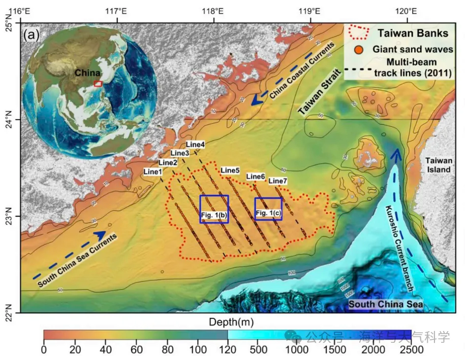
这个图的地形数据很精细,因为我画的图没展示这么精细。
底图海图可以画,然后左上角放个球形地图:
写成函数可以进行调用:
add_sphere1(cmap)
cmap指的是colormap;
调用格式: 先设置位置,在添加colormap,在调整视角即可。
%% %% add sphere  set position
axes('position',[0.02 0.49 0.42 0.42])
% add colormap
cmap=load('MPL_terrain.txt');
add_sphere1(cmap)
view(40,25);% view angles
% view(x,y);% x 控制左右旋转,y控制上下旋转。
结果展示:
图片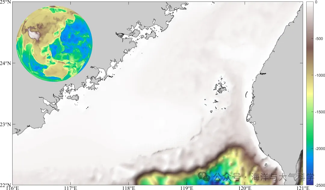
图片
图片
图片
代码:
底图海图
.rtcContent { padding: 30px; } .lineNode {font-size: 12pt; font-family: "Times New Roman", Menlo, Monaco, Consolas, "Courier New", monospace; font-style: normal; font-weight: normal; }
clc;clear;close all
% read data
file='F:\data\etopo\etopo1.nc';
lon=double(ncread(file,'x'));
lat=double(ncread( file,'y'));
h=double(ncread(file,'z'));
% 选定区域南海%
area  =[116 121 22 25];
ln =find(lon>=area(1)&lon<=area(2));
la=find(lat>=area(3)&lat<=area(4));
lon = lon(ln);
lat  = lat(la);
H = h(ln,la);
[x,y]=meshgrid(lon,lat);
x=x'; y=y';
%% %%m_pcolor画出了区域的等深线图
close all
figure;
set(0,'defaultfigurecolor','w')
set(gcf,'position',[50 50 1200 900])
m_proj('Miller','lon',[area(1) area(2)],'lat',[area(3) area(4)]);
caxis([-2500 0])% 这些必须放在m_shaderelief的前面,不然不可用
colorbar
cmap=load('MPL_terrain.txt');% add colormap
m_shadedrelief(lon,lat,H',cmap);
m_gshhs_c('patch',[0.8 0.8 0.8]);
m_grid('linest','none','xtick',[116:1:121],'ytick',[22:25],'tickdir','in',...
    'FontName','Times new roman','FontSize',12,'color','k','box','on');%box on off and fancy;
m_shadedrelief.m

.rtcContent { padding: 30px; } .lineNode {font-size: 12pt; font-family: "Times New Roman", Menlo, Monaco, Consolas, "Courier New", monospace; font-style: normal; font-weight: normal; }
function  [Truecol,x,y]=m_shadedrelief(x,y,Z,cmap,varargin)
% M_SHADEDRELIEF Shaded relief topography in an image
%  M_SHADEDRELIEF(X,Y,Z) presents a shaded relief topography, as would
%  be seen if a 3D model was artifically lit from the side. Slopes
%  facing the light are lightened, and slopes facing away from the
%  light are darkened. X and Y are horizontal and vertical coordinate
%  VECTORS, and these should be in the same units as the height Z
%  (e.g., all in meters), otherwise the slope angle calculations will be
%  in error.
%
%  Usage notes:
%
%  (1) M_SHADEDRELIEF is a replacement for a low-level call to IMAGE
%  displaying a true-colour image so it MUST be preceded by COLORMAP and
%  CAXIS calls.
%
%  (2) Gradients have to be calculated, so Z should be a data-type accepted
%   by Matlab's GRADIENT function (currently double and single).
%   If Z is (e.g.) 'int8', or some other data-type you must use
%   M_SHADED_RELIEF(X,Y,double(Z))
%
%  (3) M_SHADEDRELIEF probably is most useful as a backdrop to maps with
%  a rectangular outline box - either a cylindrical projection, or some
%  other projection with M_PROJ(...'rectbox','on').
%
%  (4) Finally, the simplest way of not running into problems:
%     - if your elevation data is in LAT/LON coords (i.e. in a matrix where
%       each row has points with the same latitude, and each column has points
%       with the same longitude), use
%                  M_PROJ('equidistant cylindrical',...)
%     - if your elevation data is in UTM coords (meters E/N), i.e. in a matrix
%       where each row has the same UTM northing and the each column has the
%       same UTM easting, use
%                  M_PROJ('utm',....)
%
%  M_SHADEDRELIEF(...,'parameter',value) lets you set various properties.
%  These are:
%       'coords' : Coordinates of X/Y/Z:
%                     'geog' for lat/lon, Z meters,  (default)
%                     'map'  for X/Y map coordinates, Z meters
%                     'Z' if X/Y/Z are all in same units (e.g., meters)
%       'lightangle' : true direction (degrees) of light source (default
%                      -45, i.e. from the north-west)
%       'gradient': Shading effects increase with slope angle
%                   until slopes reach this value (in degrees), and are
%                   held constant for higher slopes (default 10). Reduce
%                   for smoother surfaces.
%       'clipval' : Fractional change in shading for slopes>='gradient'.
%                  0 means no change, 1 means saturation to white or black
%                  if slope is facing directly towards or away from light
%                  source, (default 0.9).
%       'nancol'  : RGB colour of NaN values (default [1 1 1]);
%       'lakecol' : RGB colour of lakes (flat sections) (default NaN)
%                   If set to NaN lakes are ignored.
%
%   IM=M_SHADEDRELIEF(...) returns a handle to the image.
%
%   [SR,X,Y]=m_SHADEDRELIEF(...) does not create an image but only returns
%   the  true-color matrix SR of the shaded relief, as well as the X/Y
%   vectors needed to display it.
%
%   Example:
%           load topo
%           subplot(2,1,1);  % Example without it
%           imagesc(topolonlim,topolatlim,topo);
%           caxis([-5000 5000]);
%           colormap([m_colmap('water',64);m_colmap('gland',64)]);
%           set(gca,'ydir','normal');
%
%           subplot(2,1,2);  % Example with it
%           caxis([-5000 5000]);
%           colormap([m_colmap('water',64);m_colmap('gland',64)]);
%           m_shadedrelief(topolonlim,topolatlim,topo,'gradient',5e2,'coord','Z');
%           axis tight
%
% Rich Pawlowicz (rich@eoas.ubc.ca) Dec/2017
%
% This software is provided "as is" without warranty of any kind. But
% it's mine, so you can't sell it.
%
% Changes:
% Jan/2018 - changed outputs for flexibility
%            and added 'map' coordinate handling
% Mar/2019 - added alphamapping for out-of-map areas, started using colormap
%            local to AXES not to FIGURE.
% Apr/2019 - some parts relied on the ones-expansion; went back to meshgrid
%            for compatibility with older matlab versions (thanks P. Grahn)
% Oct/2020 - added info about how input Z must be a double
global MAP_PROJECTION MAP_VAR_LIST
lighthead=-45;
gradfac=10;
clipval=.9;
nancol=[1 1 1];
lakecol=NaN; %[.7 .9 1];
geocoords='geog';
scfac=6400000;  % Used for geo coordinates if on sphere radius 1
while ~isempty(varargin)
    switch lower(varargin{1}(1:3))
        case 'coo'
            switch lower(varargin{2}(1))
                case 'g'
                    geocoords='geog';
                case 'm'
                    geocoords='map';
                case {'z','u'}
                    geocoords='z';
                otherwise
                    error('Unknown coordinate specification');
            end
        case 'lig'
            lighthead=varargin{2};
        case 'gra'
            gradfac=varargin{2};
        case 'cli'
            clipval=varargin{2};
        case 'nan'
            nancol=varargin{2};
        case 'lak'
            lakecol=varargin{2};
        otherwise
            error(['m_shadedrelief: Unknown option: ' varargin{1}]);
    end
    varargin(1:2)=[];
end
% All kinds of issues dealing with coords:
% First, we need VECTOR x/y as an input to gradient function.
if isvector(x) && size(x,2)==1
    x=x';
elseif ~isvector(x)       % Can't be a matrix
    error('Input X must be a VECTOR');
end
if isvector(y) && size(y,1)==1
    y=y';
elseif ~isvector(y)
    error('Input Y must be a VECTOR');
end
%  Now handle the case if we just give a starting and an ending point
if length(x)==2
    x=linspace(0,1,size(Z,2))*diff(x)+x(1);
end
if length(y)==2
    y=linspace(0,1,size(Z,1))'*diff(y)+y(1);
end
if strcmp(geocoords,'geog')                           %  If its Lat/Long points
    % Have to have initialized a map first
    if isempty(MAP_PROJECTION)
        disp('No Map Projection initialized - call M_PROJ first!');
        return;
    end
    % Convert to X/Y
    [X,Y]=m_ll2xy(x(1,:),repmat(mean(y(:,1)),1,size(x,2)),'clip','off');
    [X2,Y2]=m_ll2xy(repmat(mean(x(1,:)),size(y,1),1),y(:,1),'clip','off');
    x=X;
    y=Y2;
end
% Note - 'image' spaces points evenly, so we should just check that they
% are even otherwise the image won't line up with coastlines...
if max(abs( x - linspace(x(1),x(end),length(x)) ) )/abs(x(end)-x(1)) >.005
    warning(['********** Image will be distorted in X direction!! use M_IMAGE to re-map? *************']);
end
if max(abs( y - linspace(y(1),y(end),length(y))' ) )/abs(y(end)-y(1)) >.005
    warning(['********** Image will be distorted in Y direction!! use M_IMAGE to re-map? *************']);
end
% Convert colours to uint8s
if all(nancol<=1)
    nancol=uint8(nancol*255);
end
% Convert colours to uint8s
if all(lakecol<=1)
    lakecol=uint8(lakecol*255);
end
% Get caxis
clims=caxis;
if all(clims==[0 1])   % Not set
    clims=[min(Z(:)) max(Z(:))];
end
% Get colormap for the current axes
% cmap1=load('GMT_drywet1.mat');
% cmap1 =(cmap1.raw_new);
% cc=colormap((cmap1));
if isempty(cmap)
    cmap=load('MPL_terrain.txt');
else
    cmap = cmap;
end
cc=colormap((cmap));
% cc=colormap(gca);
cc2=round(cc*255);  % we need these in 0-255 range to get Truecolor
lcc=size(cc,1);
%inan=isnan(Z);
% Get slopes
% If we are using a normal ellipsoid we need to rescale
% x/y to get true slope angles
if ~isfloat(Z)
    warning('Your input Z matrix must be floating point');
end
if  (strcmp(geocoords,'map') || strcmp(geocoords,'geog')) && strcmp(MAP_VAR_LIST.ellipsoid,'normal')
    scfac=6370997;
    [Fx,Fy]=gradient( Z, x*scfac, y*scfac);
else
    [Fx,Fy]=gradient( Z, x, y);
end
% Find NaN
[inan,jnan]=find(isnan(Z) | isnan(Fx) | isnan(Fy) );
% Probable lakes
[islake,jlake]=find(Fx==0 & Fy==0);
% Convert z levels into a colormap index.
% Some iteration to discover the exact formula that matlab uses for mapping to
% color indices (from 1 to lcc)
%idx=min( floor( min(max( (Z-clims(1))/(clims(2)-clims(1)),0) ,1 )*lcc )+1,lcc);
idx=max(min( floor(   (Z-clims(1))/(clims(2)-clims(1))*lcc  )+1  ,lcc),1);
% The slope angle relative to the light direction in degrees.
Fnw=atand(imag(-(Fx+i*Fy)*exp(i*lighthead*pi/180)));
%Put an upper and lower limit on the angles
%%Fnw=min(clipval,max(-clipval,Fnw/gradfac));
Fnw=clipval*tanh(Fnw/gradfac);
% Now get the colormap for each pixel and scale the RGB value 'c'.
% If the correction is -0.1 then scale  c*(1 - |-0.1|)
% If the correction is  0.1 then scale  c*(1 - |+0.1|) + 0.1*255
%depending on the slope.
%Truecol=uint8(max(0,min(255,   reshape([cc2(idx,:)],[size(idx) 3]).*repmat(1-abs(Fnw),1,1,3)+repmat(255*Fnw.*(Fnw>0),1,1,3) ) ));
Truecol=uint8( reshape([cc2(idx,:)],[size(idx) 3]).*repmat(1-abs(Fnw),1,1,3)+repmat(255*Fnw.*(Fnw>0),1,1,3) ) ;
%Truecol=uint8(max(0,min(255,   reshape([cc2(idx,:)],[size(idx) 3]).*repmat(1+Fnw/gradfac,1,1,3) ) ));
% Colour Lakes
if any(islake) && isfinite(lakecol(1))
    Truecol(sub2ind(size(Truecol),islake,jlake,  ones(size(islake))))=lakecol(1);
    Truecol(sub2ind(size(Truecol),islake,jlake,1+ones(size(islake))))=lakecol(2);
    Truecol(sub2ind(size(Truecol),islake,jlake,2+ones(size(islake))))=lakecol(3);
end
% Colour the NaNs
if any(inan)
    Truecol(sub2ind(size(Truecol),inan,jnan,  ones(size(inan))))=nancol(1);
    Truecol(sub2ind(size(Truecol),inan,jnan,1+ones(size(inan))))=nancol(2);
    Truecol(sub2ind(size(Truecol),inan,jnan,2+ones(size(inan))))=nancol(3);
end
if strcmp(geocoords,'map')   % Have to "make invisible" the points outside the map limits.
    [xm,ym]=meshgrid(x,y);
    [HLG,HLT]=m_xy2ll(xm,ym);
    % Find pixels outside the limits of the actual map (if the boundary
    % isn't a rectangle)
    if strcmp(MAP_VAR_LIST.rectbox,'off')
        [I,J]=find(HLT<MAP_VAR_LIST.lats(1) | HLT>MAP_VAR_LIST.lats(2) | HLG<MAP_VAR_LIST.longs(1) | HLG>MAP_VAR_LIST.longs(2));
    elseif strcmp(MAP_VAR_LIST.rectbox,'circle')
        R=(xm.^2 +ym.^2);
        [I,J]=find(R>MAP_VAR_LIST.rhomax.^2);
    else
        I=[];J=[];
    end
    backcolor=uint8(get(gcf,'color')*255);
    if any(I)                          % if some pixels are outside the map area
        for k=1:3
            IJ=sub2ind(size(Truecol),I,J,repmat(k,size(I)));
            Truecol(IJ)=backcolor(k);           % Set them to the background colour
        end
    end
else
    I=[];J=[];
end
if nargout<=1
    if any(I)  % make pixels outside the map area transparent, if needed.
        alphadata=  ones(size(Truecol,1),size(Truecol,2),'logical');
        IJ=sub2ind(size(alphadata),I,J);
        alphadata(IJ)=0;
        Truecol=image('xdata',x,'ydata',y,'cdata',Truecol,'alphadata',alphadata,'tag','m_shadedrelief');
    else
        Truecol=image('xdata',x,'ydata',y,'cdata',Truecol,'tag','m_shadedrelief');
    end
end
add_sphere1
.rtcContent { padding: 30px; } .lineNode {font-size: 12pt; font-family: "Times New Roman", Menlo, Monaco, Consolas, "Courier New", monospace; font-style: normal; font-weight: normal; }
function add_sphere1(cmap)
load topo topo topomap1    % load data
x = 0:359;                                % longitude
y = -89:90;                               % latitude
[X1,Y1]=meshgrid(x,y);
x1 = 0:0.1:360;
y1=-89:0.1:90;
[X,Y]=meshgrid(x1,y1);
topo_new = griddata(X1,Y1,topo,X,Y);
% figure;
% set(0,'defaultfigurecolor','w')
% set(gcf,'position',[50 50 1200 900])
[x,y,z] = sphere(100);          % create a sphere
s = surface(x,y,z);            % plot spherical surface
s.FaceColor = 'texturemap';    % use texture mapping
s.CData = topo_new;                % set color data to topographic data
s.EdgeColor = 'none';          % remove edges
s.FaceLighting = 'gouraud';    % preferred lighting for curved surfaces
s.SpecularStrength = 0.4;      % change the strength of the reflected light
if isempty(cmap)
    cmap=load('MPL_terrain.txt');
else
    cmap = cmap;
end
colormap(cmap)
% light('Position',[1 0 1])     % add a light
axis square off                % set axis to square and remove axis
view([30,10])                 % set the viewing angle

![[密码学实战]密评考试训练系统v1.0程序及密评参考题库(获取路径在文末)](https://i-blog.csdnimg.cn/direct/b5725199526a44edba1e139533e708d8.png#pic_center)