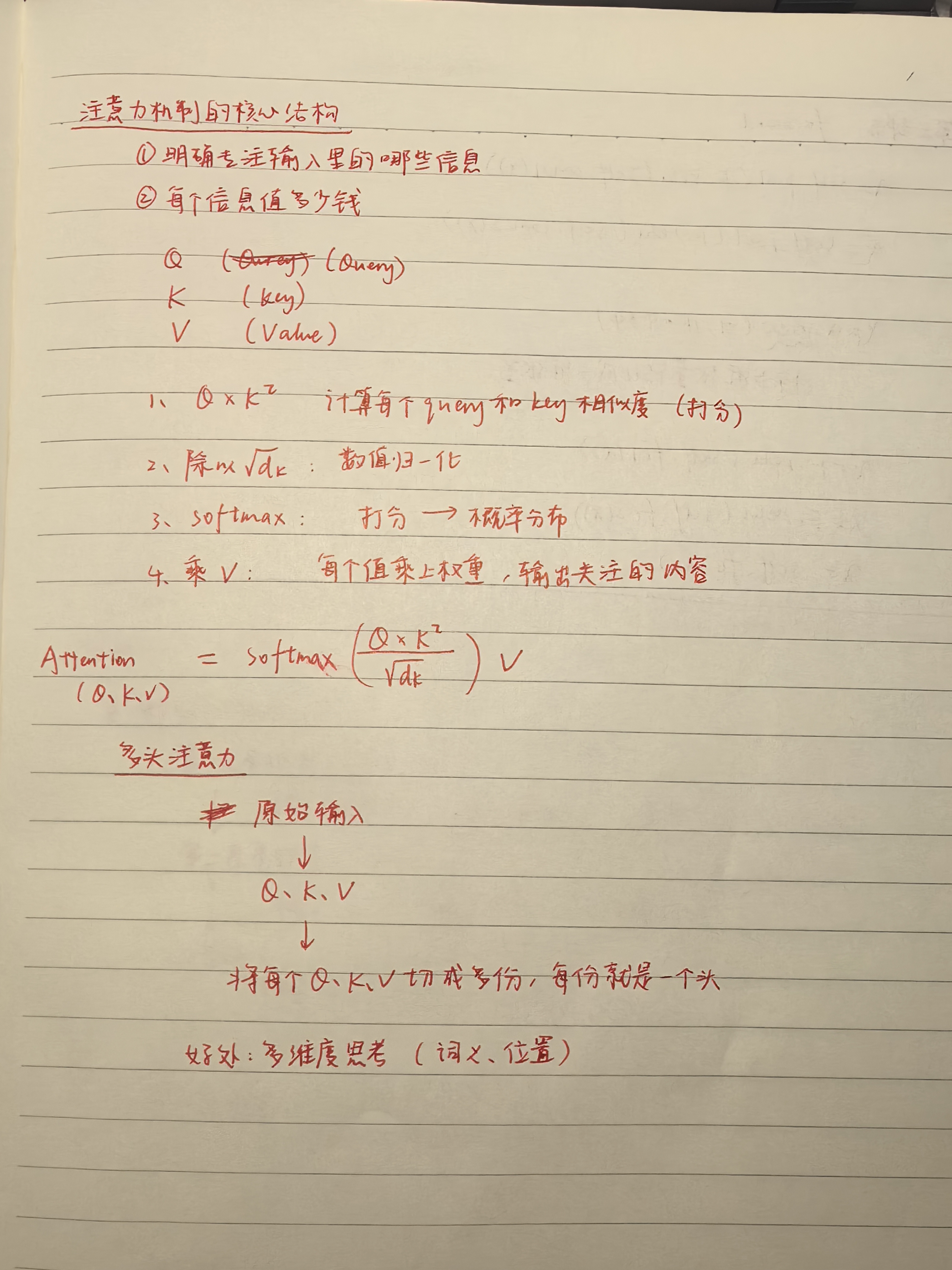
单头注意力机制
import torch
import torch.nn.functional as F

def scaled_dot_product_attention(Q, K, V):
    # Q: (batch_size, seq_len, d_k)
    # K: (batch_size, seq_len, d_k)
    # V: (batch_size, seq_len, d_v)
batch_size: 一次输入的句子数。
seq_len: 每个句子的词数。
d_model: 每个词的表示维度,比如 512。
d_k 是 Query 和 Key 向量的维度。
   # 计算点积 QK^T 并进行缩放
   d_k = Q.size(-1)  # 获取 Key 的维度
   scores = torch.matmul(Q, K.transpose(-2, -1)) / torch.sqrt(torch.tensor(d_k, dtype=torch.float32))
Q = torch.tensor([
[[1.0, 0.0], # The
[0.0, 1.0], # cat
[1.0, 1.0]] # sat
]) # shape = (1, 3, 2) batch=1, seq_len=3, d_k=2
获取最后一维(每个词的维度),这里是 2
(新例子)原本 Q 和 K 都是形状 (1, 3, 2),即 batch=1,3个词,每个词2维。
matmul 就是 矩阵乘法
transpose(-2, -1) 表示 交换最后两个维度
Q = (1, 3, 4):1 个样本,3 个词,每个词是 4 维向量
K = (1, 3, 4):同样 3 个词,每个词是 4 维向量
K.transpose(-2, -1) → (1, 4, 3)
torch.matmul(Q, K^T) → (1, 3, 4) @ (1, 4, 3) → (1, 3, 3)
    # 计算 softmax 得到注意力权重
    attention_weights = F.softmax(scores, dim=-1)  # 对最后一个维度进行 softmax
“打分矩阵”scores 变成“权重矩阵”attention_weights,决定每个词该关注谁、关注多少。
F 是 PyTorch 的一个模块,torch.nn.functional 的简称。
它提供了一大堆“函数式的操作”,比如:F.relu()、F.softmax()、F.cross_entropy()
Softmax 是一个数学函数,它把一组“任意的实数”变成“总和为 1 的概率分布”。
它会让大的值变成更大的概率,小的值变成更小的概率
所有值会被缩放到 0 到 1 之间,并且总和是 1
dim=-1 表示在最后一个维度上做 softmax。
在注意力机制中,scores 是形状 (batch_size, seq_len, seq_len),比如 (1, 3, 3)
scores = torch.tensor([[
[10.0, 2.0, -1.0], # 第一个词对其他词的打分
[5.0, 0.0, -2.0], # 第二个词对其他词的打分
[0.0, 0.0, 0.0] # 第三个词平等看待其他词
]]) # shape = (1, 3, 3)
softmax([10, 2, -1]) = [e^10, e^2, e^-1] / (e^10 + e^2 + e^-1)
e^10 ≈ 22026.5
e^2 ≈ 7.389
e^-1 ≈ 0.367
总和 ≈ 22026.5 + 7.389 + 0.367 ≈ 22034.3
所以 softmax ≈ [0.9996, 0.00033, 0.000016]
tensor([[
[0.9996, 0.0003, 0.0000],
[0.9933, 0.0066, 0.0000],
[0.3333, 0.3333, 0.3333]
]])
对 dim = -1 做 softmax
意思是:对于每个 Query 的“对别人的打分”那一行,我们做 softmax
    # 使用注意力权重对 V 进行加权求和
    output = torch.matmul(attention_weights, V)
每个 Query 位置根据它对所有词的注意力权重,对 Value 做加权平均,输出一个 2 维向量。
    return output, attention_weights

# 示例输入
batch_size, seq_len, d_k, d_v = 2, 5, 8, 8  # 批量大小、序列长度、Key 维度、Value 维度
Q = torch.randn(batch_size, seq_len, d_k)  # Query
K = torch.randn(batch_size, seq_len, d_k)  # Key
V = torch.randn(batch_size, seq_len, d_v)  # Value

output, attention_weights = scaled_dot_product_attention(Q, K, V)
print("Output shape:", output.shape)  # 输出形状应为 (batch_size, seq_len, d_v)
print("Attention weights shape:", attention_weights.shape)  # 注意力权重形状应为 (batch_size, seq_len, seq_len)
多头注意力机制
class MultiHeadAttention(nn.Module):
    def __init__(self, d_model, num_heads):
        super(MultiHeadAttention, self).__init__()
        assert d_model % num_heads == 0, "d_model must be divisible by num_heads"

        self.d_model = d_model  # 输入向量维度 = 8
        self.num_heads = num_heads  # 头的数量
        self.depth = d_model // num_heads  # 每个头的维度

        # 定义线性变换矩阵
        self.W_Q = nn.Linear(d_model, d_model)  # Query 线性变换
        self.W_K = nn.Linear(d_model, d_model)  # Key 线性变换
        self.W_V = nn.Linear(d_model, d_model)  # Value 线性变换
        self.W_O = nn.Linear(d_model, d_model)  # 输出线性变换
Linear 是 PyTorch 里的线性变换层(全连接层 / 仿射变换)
    def split_heads(self, x, batch_size):
        # 将输入张量分割为多个头
        # 输入形状: (batch_size = 2, seq_len = 2, d_model = 16)
        # 输出形状: (batch_size2, num_heads8, seq_len2, depth = 2)
        x = x.view(batch_size, -1, self.num_heads, self.depth)
        return x.permute(0, 2, 1, 3)
所以要把每个 16 维向量,切分成 8 个头,每个头是 2 维,方便后面“并行注意力”。
view:原始张量先展平成一维向量 然后按给的新形状,按行依次填进去
-1 在 view 中的作用是–让 PyTorch 自动推导这一维的大小,只要其余维度的乘积是对得上的
permute:维度重新排列
    def forward(self, Q, K, V):
        batch_size = Q.size(0)

        # 线性变换
        Q = self.W_Q(Q)  # (batch_size, seq_len, d_model)
        K = self.W_K(K)  # (batch_size, seq_len, d_model)
        V = self.W_V(V)  # (batch_size, seq_len, d_model)

        # 分割为多个头
        Q = self.split_heads(Q, batch_size)  # (batch_size, num_heads, seq_len, depth)
        K = self.split_heads(K, batch_size)  # (batch_size, num_heads, seq_len, depth)
        V = self.split_heads(V, batch_size)  # (batch_size, num_heads, seq_len, depth)

        # 计算每个头的注意力
        # 就是使用上述的注意力的公式
        scaled_attention, _ = scaled_dot_product_attention(Q, K, V)

        # 拼接多个头的输出
        # 返回一个内存连续的张量副本
        scaled_attention = scaled_attention.permute(0, 2, 1, 3).contiguous()  # (batch_size, seq_len, num_heads, depth)

        concat_attention = scaled_attention.view(batch_size, -1, self.d_model)  # (batch_size, seq_len, d_model)
你把 8 个头的 summary 合并,就是一份完整的理解(512 维)
        # 最终线性变换
        output = self.W_O(concat_attention)  # (batch_size, seq_len, d_model)
concat_attention = [1.0, 2.0, 3.0, 4.0]
有个线性层(随机初始化):
W_O = [
[0.1, 0.2, 0.3, 0.4],
[0.5, 0.6, 0.7, 0.8],
[0.9, 1.0, 1.1, 1.2],
[1.3, 1.4, 1.5, 1.6]
]
执行线性变换:
output = concat_attention @ W_O^T
        return output

# 示例输入
batch_size, seq_len, d_model, num_heads = 2, 5, 8, 4  # 批量大小、序列长度、模型维度、头数量
Q = torch.randn(batch_size, seq_len, d_model)  # Query
K = torch.randn(batch_size, seq_len, d_model)  # Key
V = torch.randn(batch_size, seq_len, d_model)  # Value

# 实例化多头注意力
mha = MultiHeadAttention(d_model, num_heads)

# 前向传播
output = mha(Q, K, V)
print("Output shape:", output.shape)  # 输出形状应为 (batch_size, seq_len, d_model)
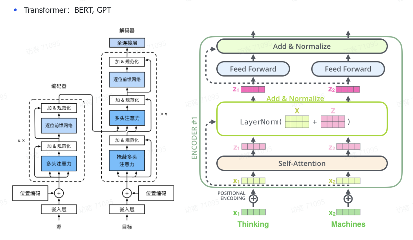
左图:
编码器(Encoder):
左边一列是 Encoder,作用是处理输入序列(比如一句话)。
每一层包含:
多头注意力(Self-Attention):让每个词关注上下文中其他词的信息(注意力机制的核心)。
前馈神经网络(Feed Forward):对每个词做单独的非线性变换。
加法残差连接 + LayerNorm(加 & 规范化):提升训练稳定性。
👉 这些结构堆叠 n 层,输出的是编码后的向量表示。
解码器(Decoder):
用于生成输出序列(例如翻译一句话)。
每层包括:
掩蔽多头注意力(Masked Multi-Head Attention):阻止看到未来词,适用于生成任务。
跨注意力(对编码器输出):Decoder 的词可以关注 Encoder 的词。
前馈网络 + 加法规范化:和 Encoder 一样。
右图
输入:x₁ = “Thinking”, x₂ = “Machines”
第一步:Self-Attention
这里会用多头注意力(Q, K, V 都来自同一个输入)
计算每个词该关注谁,输出一个“上下文相关的向量”
第二步:残差连接 + LayerNorm
text
复制
编辑
Z1 = Self-Attention(x)
LayerNorm(x + Z1)
原始输入 x 和 Attention 输出相加,再归一化
保证梯度稳定,避免训练时梯度爆炸或消失
第三步:Feed Forward
一个两层的全连接网络(对每个位置独立操作)
x = Linear → ReLU → Linear
再加一次残差 + LayerNorm:
Z2 = FeedForward()
LayerNorm(Z1 + Z2)
第四步:
输出是:编码后的向量序列(包含上下文信息),可以喂给 Decoder 或下游任务。


![[c语言日寄]免费文档生成器——Doxygen在c语言程序中的使用](https://i-blog.csdnimg.cn/direct/556c5a2c798045c6aeacdb24ace3e13e.gif#pic_center)