Tensorflow2.0
有深度学习基础的建议直接看class3
class1
介绍
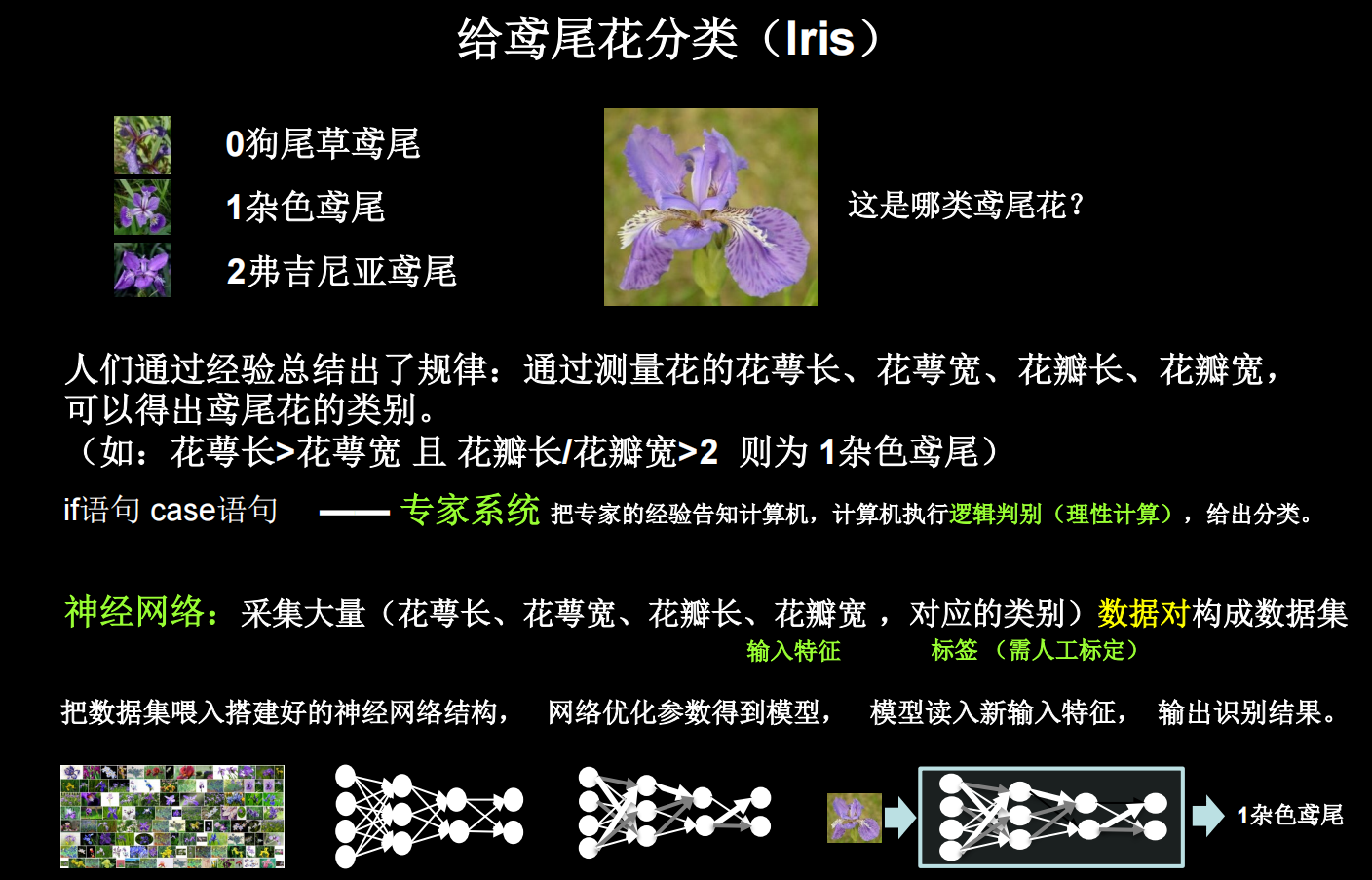
人工智能3学派
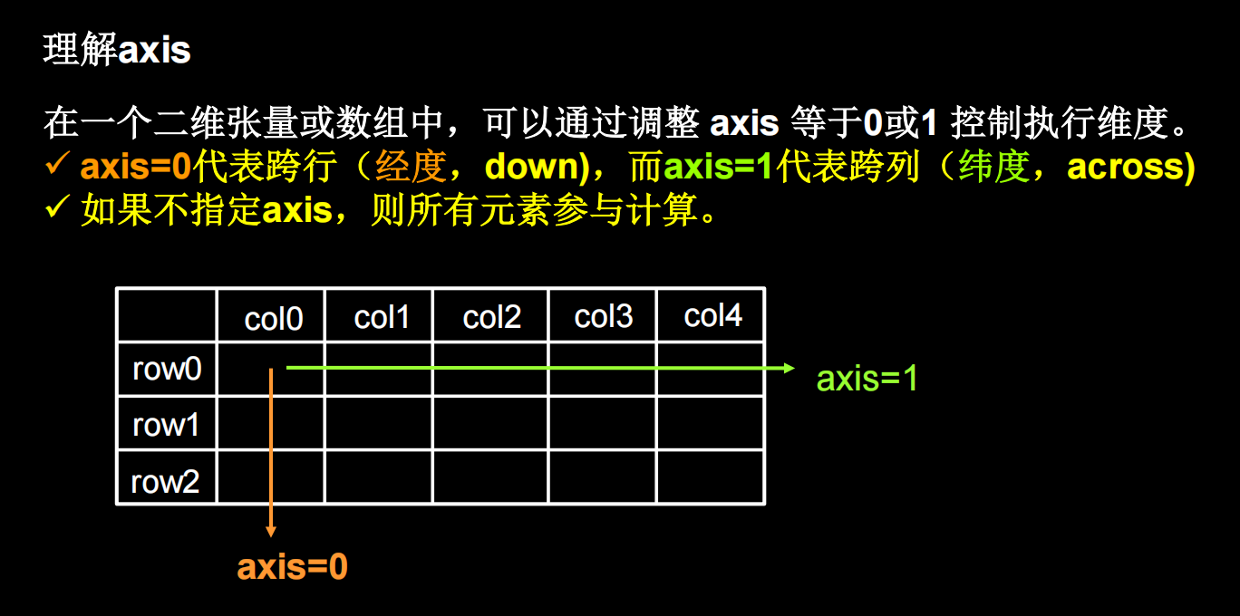
行为主义:基于控制论,构建感知-动作控制系统。(控制论,如平衡、行走、避障等自适应控制系统)
符号主义:基于算数逻辑表达式,求解问题时先把问题描述为表达式,再求解表达式。(可用公式描述、实现理性思维,如专家系统)
连接主义:仿生学,模仿神经元连接关系。(仿脑神经元连接,实现感性思维,如神经网络)
行为主义的例子,让机器人单脚站立,通过感知要摔倒的方向控制两只手的动作,保持身体的平衡,这就构建了一个感知-动作控制系统
张量生成

TensorFlow的数据类型
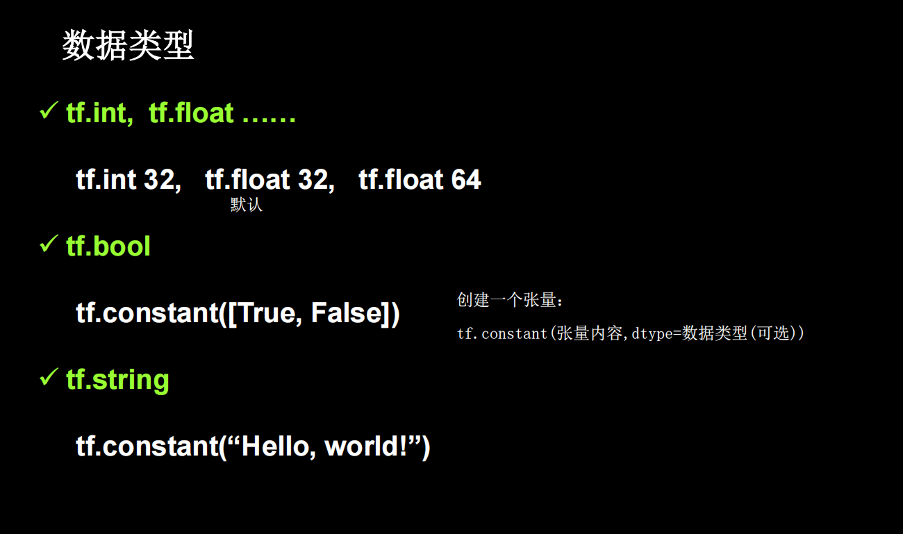
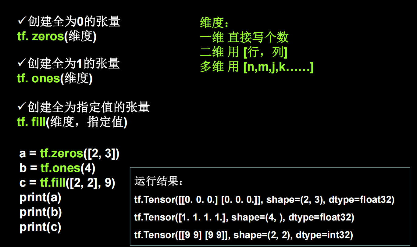
创建一个张量
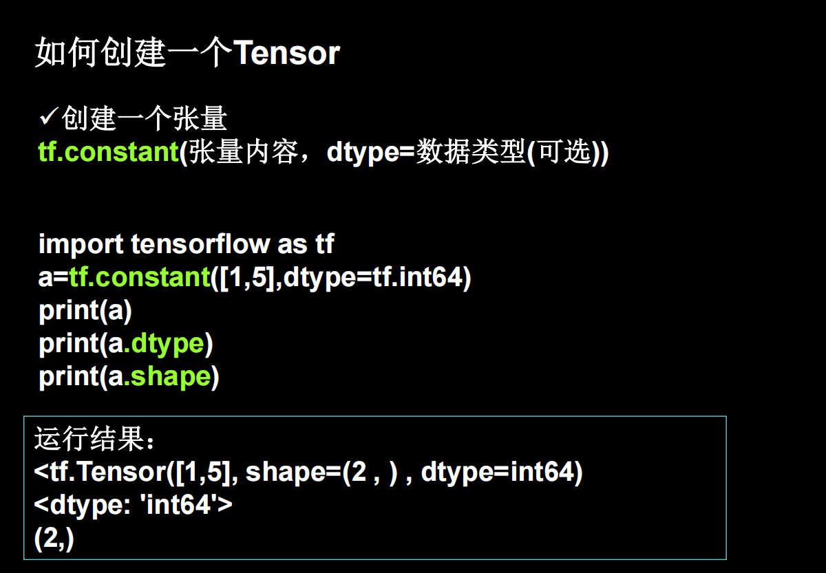
shape括号中隔开了几个数字,就是几维张量,上图隔开一个数字,说明是一维张量
a=tf.constant([[3,6,4],[11,56,2]],dtype=tf.int64)
print(a)
print(a.shape)
print(a.dtype)
"""
tf.Tensor(
[[ 3  6  4]
 [11 56  2]], shape=(2, 3), dtype=int64)
(2, 3)
<dtype: 'int64'>
"""
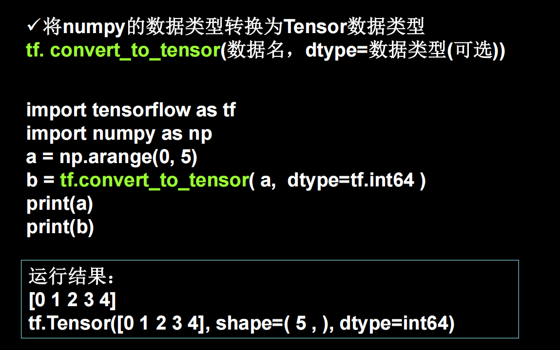
有时候数据格式是numpy
还可以直接用函数快速创建特殊的张量矩阵
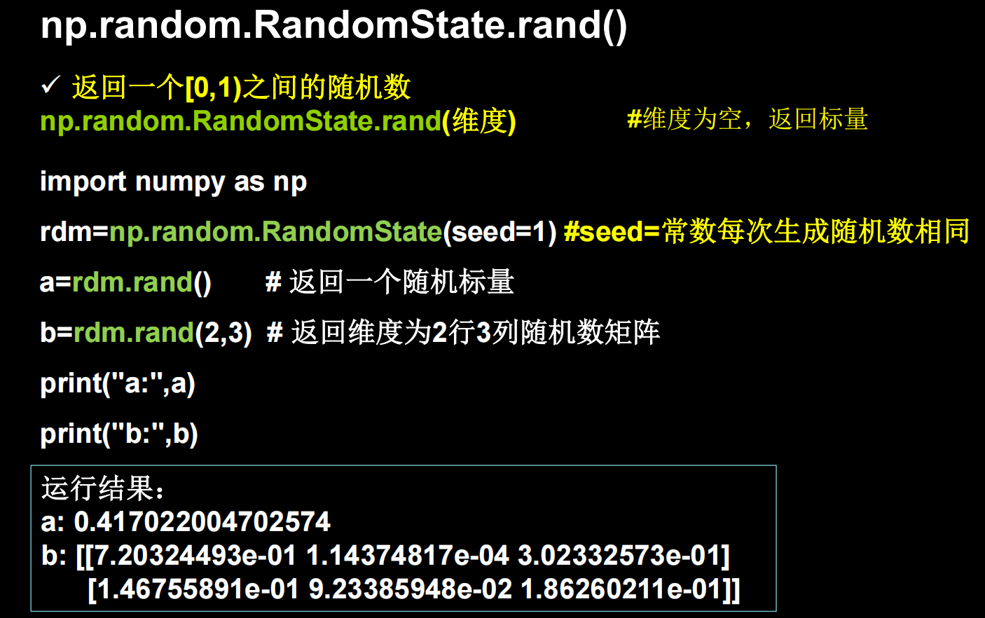
还有一些生产随机数的方法
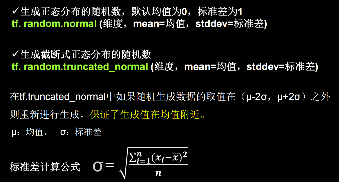
比如

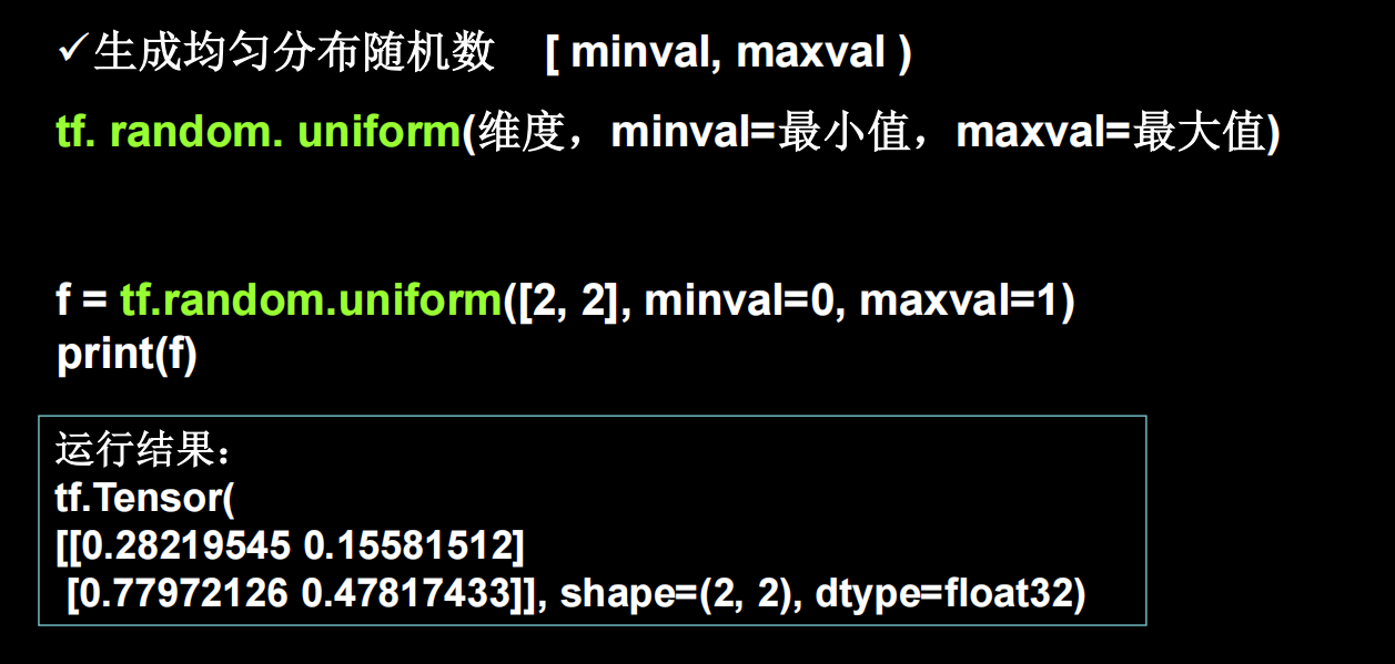
生成均匀分布随机数(注意区间是前闭后开)
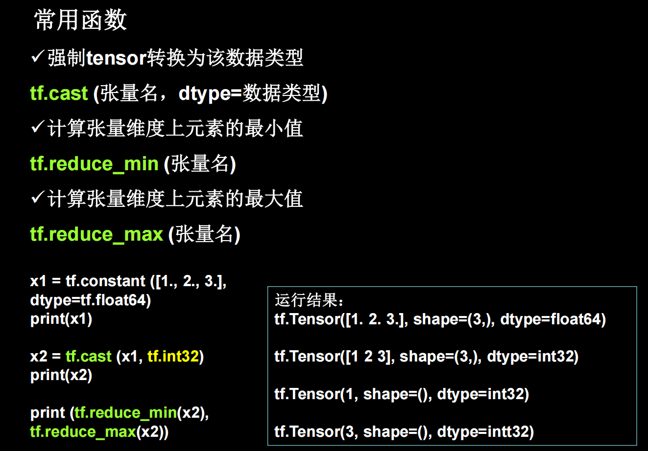
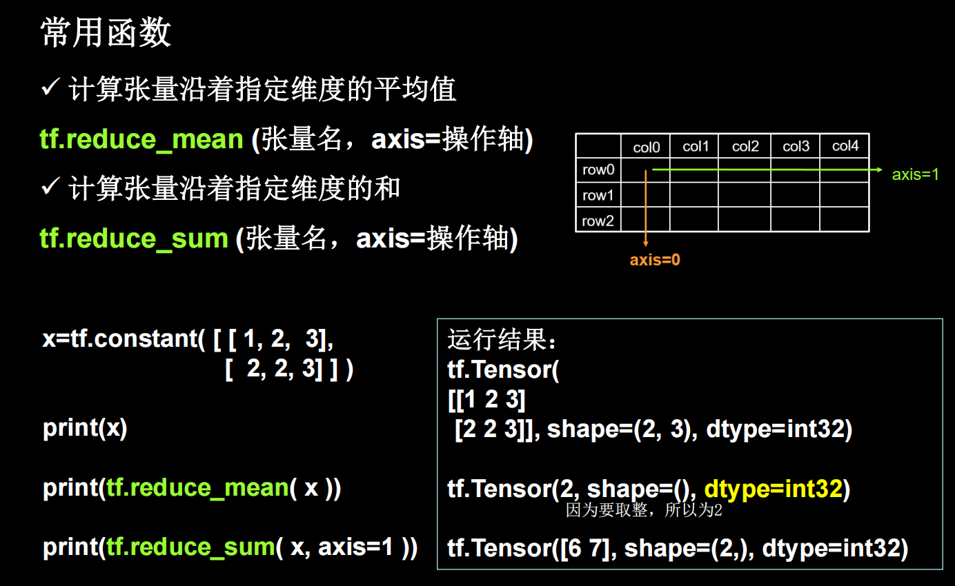
tf常用函数1
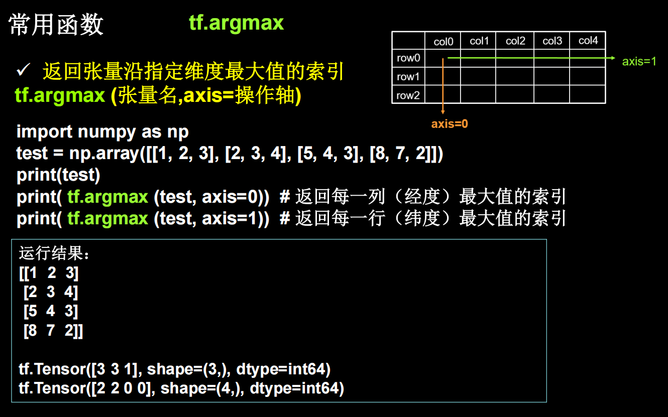
理解axis
例子
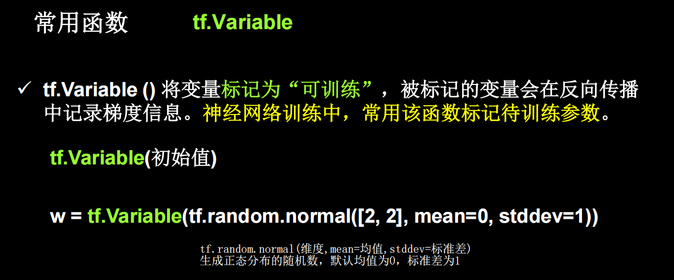
可训练的
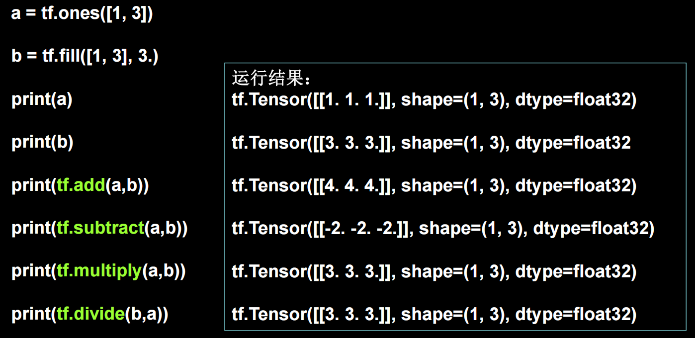
TensorFlow中的数学运算
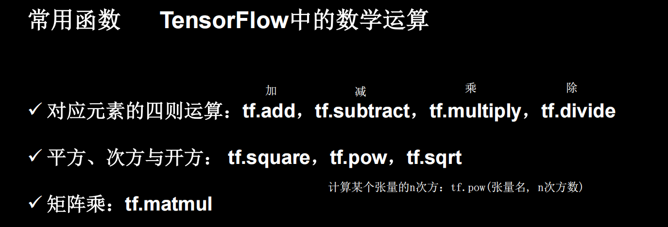
对应元素的四则运算

例子
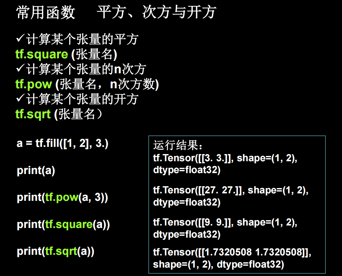
平方、次方与开方
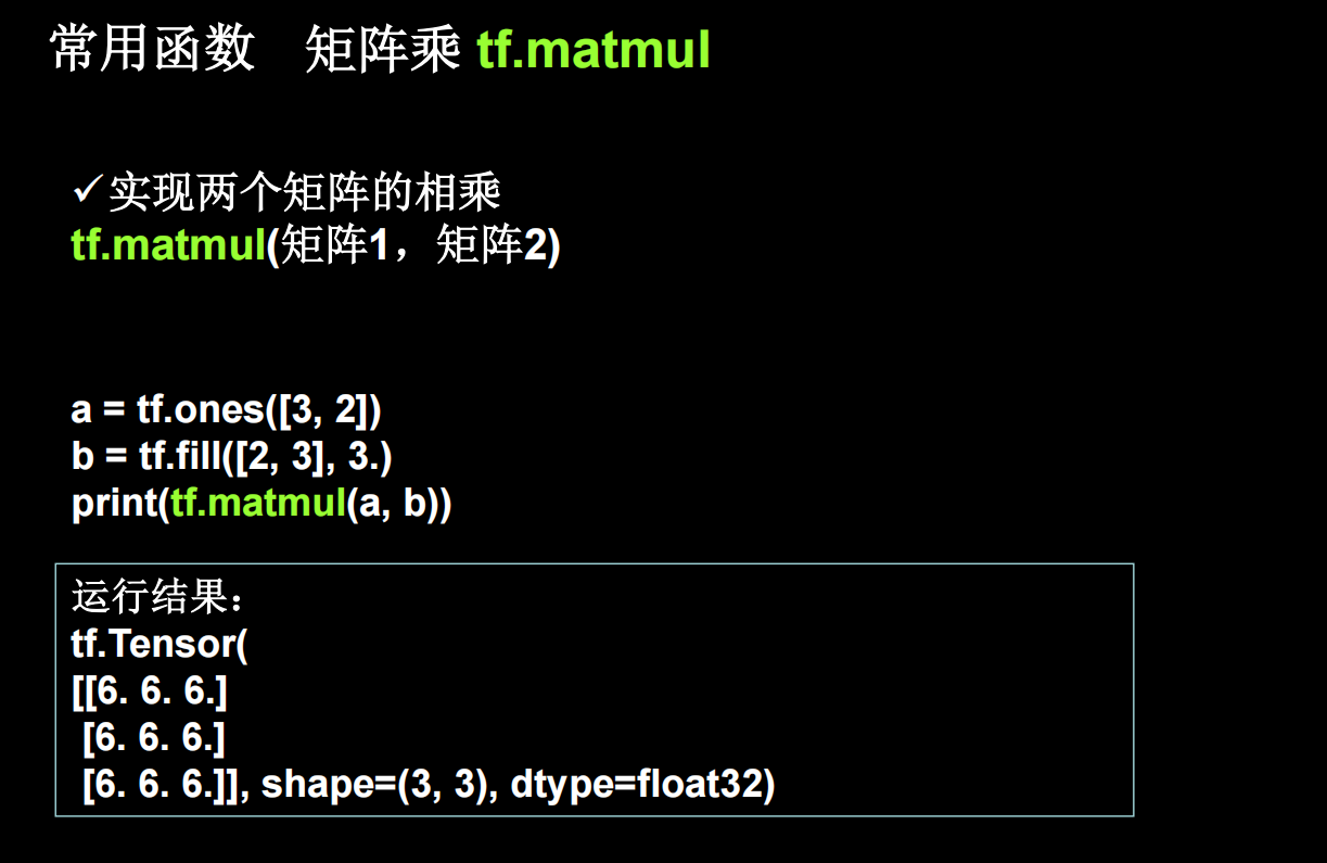
矩阵乘
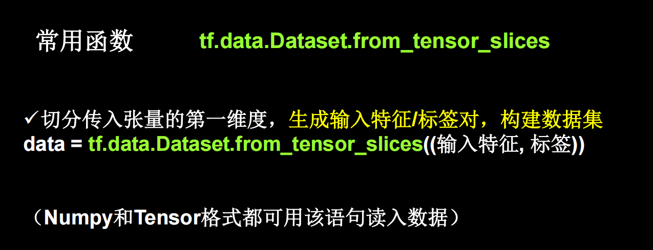
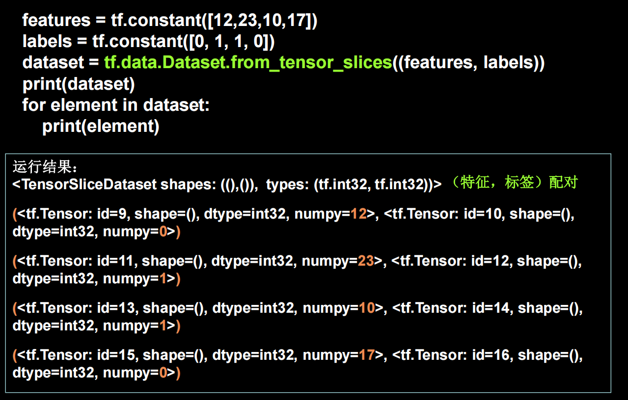
tensorflow输入数据
具体例子
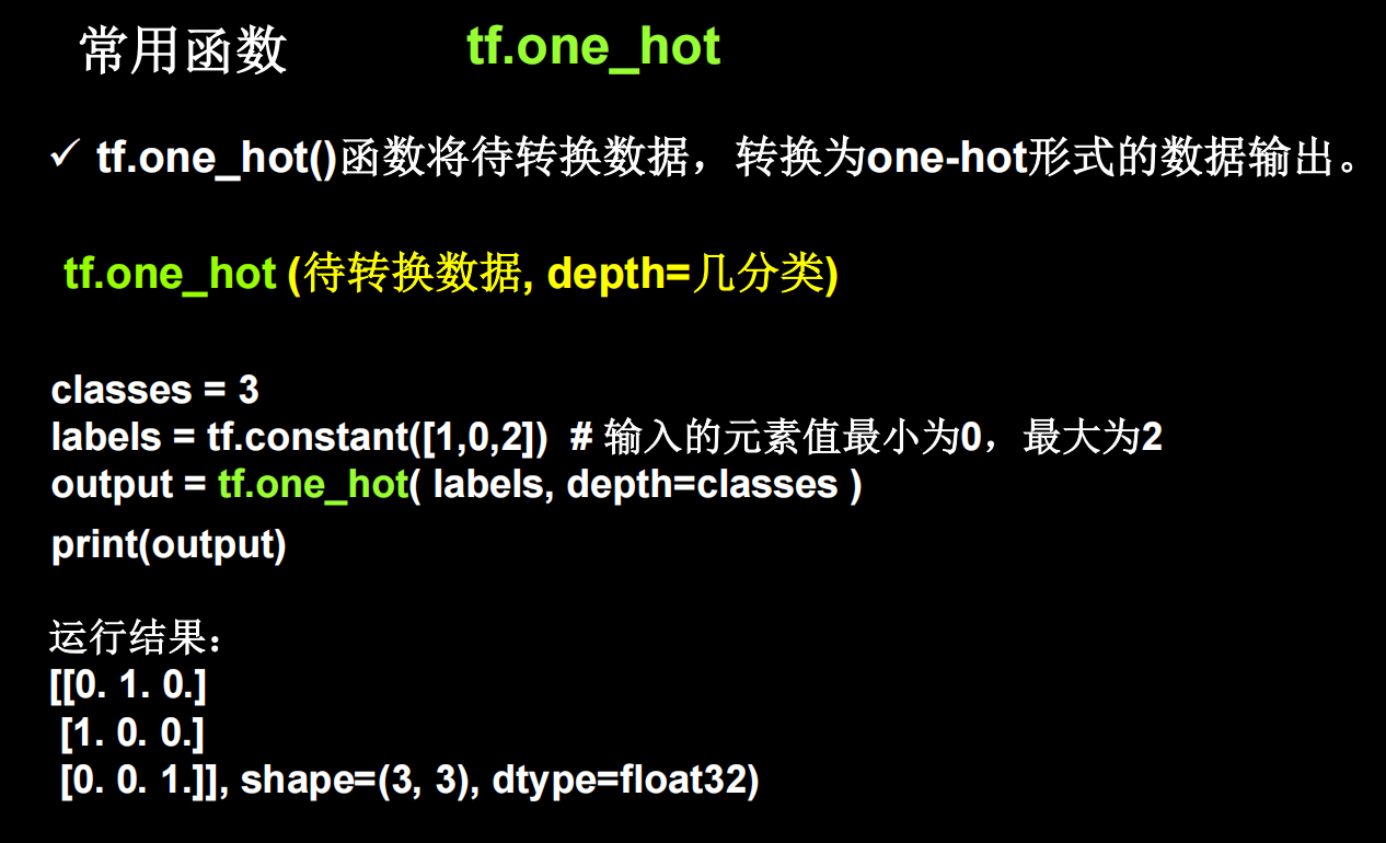
tf常用函数2
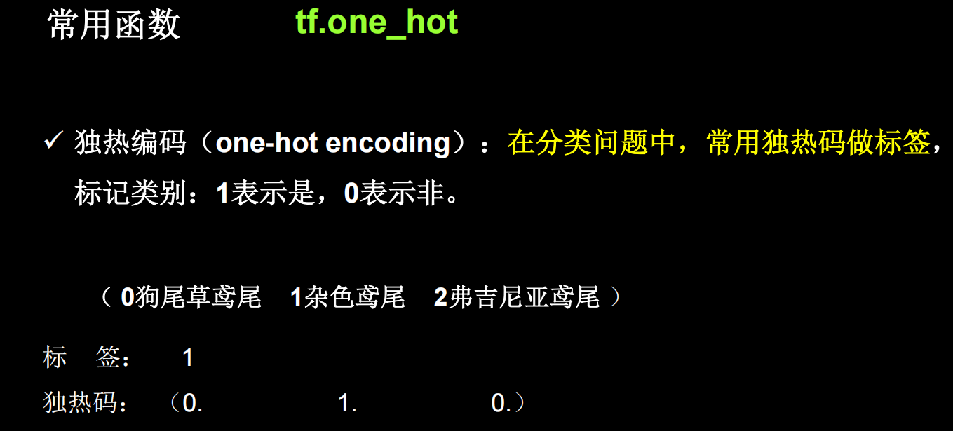
tensorflow中提供了one-hot函数
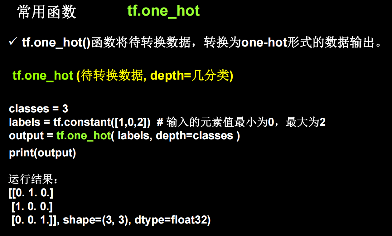
例子
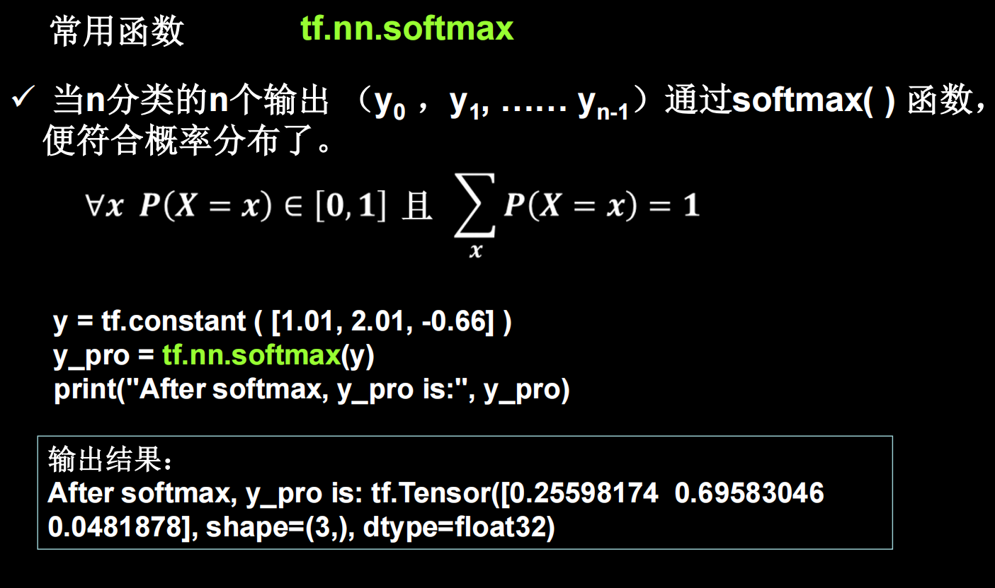
使输出符合概率分布
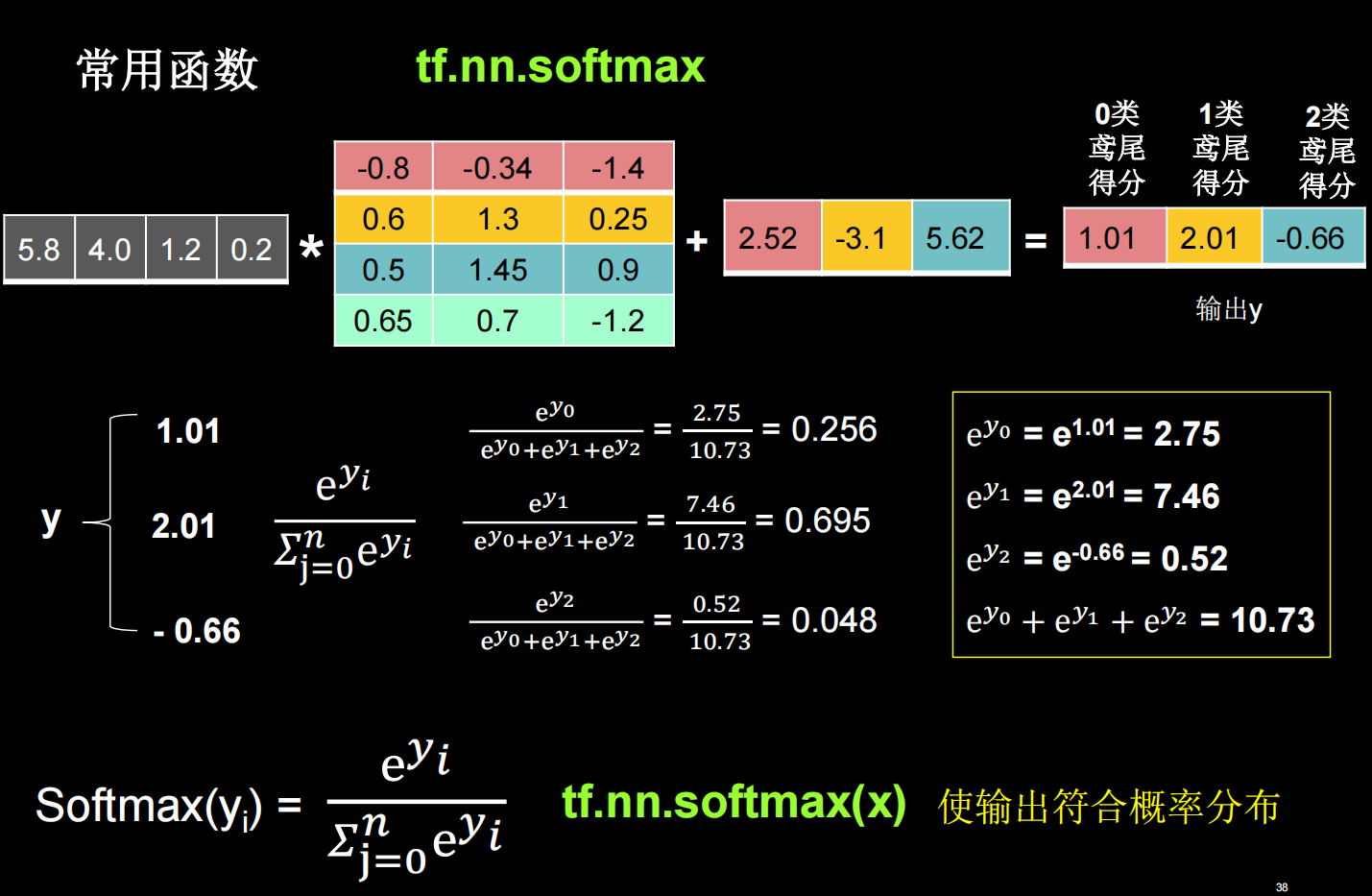
tf.nn.softmax
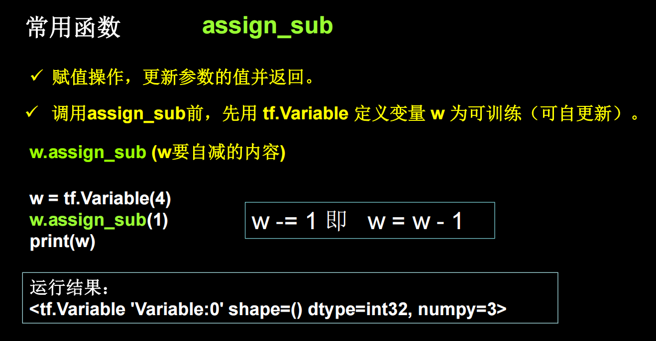
assign_sub更新参数
鸢尾花分类
# -*- coding: UTF-8 -*-
# 利用鸢尾花数据集,实现前向传播、反向传播,可视化loss曲线
# 导入所需模块
import tensorflow as tf
from sklearn import datasets
from matplotlib import pyplot as plt
import numpy as np
# 导入数据,分别为输入特征和标签
x_data = datasets.load_iris().data
y_data = datasets.load_iris().target
# 随机打乱数据(因为原始数据是顺序的,顺序不打乱会影响准确率)
# seed: 随机数种子,是一个整数,当设置之后,每次生成的随机数都一样(为方便教学,以保每位同学结果一致)
np.random.seed(116) # 使用相同的seed,保证输入特征和标签一一对应
np.random.shuffle(x_data)
np.random.seed(116)
np.random.shuffle(y_data)
tf.random.set_seed(116)
# 将打乱后的数据集分割为训练集和测试集,训练集为前120行,测试集为后30行
x_train = x_data[:-30]
y_train = y_data[:-30]
x_test = x_data[-30:]
y_test = y_data[-30:]
# 转换x的数据类型,否则后面矩阵相乘时会因数据类型不一致报错
x_train = tf.cast(x_train, tf.float32)
x_test = tf.cast(x_test, tf.float32)
# from_tensor_slices函数使输入特征和标签值一一对应。(把数据集分批次,每个批次batch组数据)
train_db = tf.data.Dataset.from_tensor_slices((x_train, y_train)).batch(32)
test_db = tf.data.Dataset.from_tensor_slices((x_test, y_test)).batch(32)
# 生成神经网络的参数,4个输入特征故,输入层为4个输入节点;因为3分类,故输出层为3个神经元
# 用tf.Variable()标记参数可训练
# 使用seed使每次生成的随机数相同(方便教学,使大家结果都一致,在现实使用时不写seed)
w1 = tf.Variable(tf.random.truncated_normal([4, 3], stddev=0.1, seed=1))
b1 = tf.Variable(tf.random.truncated_normal([3], stddev=0.1, seed=1))
lr = 0.1 # 学习率为0.1
train_loss_results = [] # 将每轮的loss记录在此列表中,为后续画loss曲线提供数据
test_acc = [] # 将每轮的acc记录在此列表中,为后续画acc曲线提供数据
epoch = 500 # 循环500轮
loss_all = 0 # 每轮分4个step,loss_all记录四个step生成的4个loss的和
# 训练部分
for epoch in range(epoch): #数据集级别的循环,每个epoch循环一次数据集
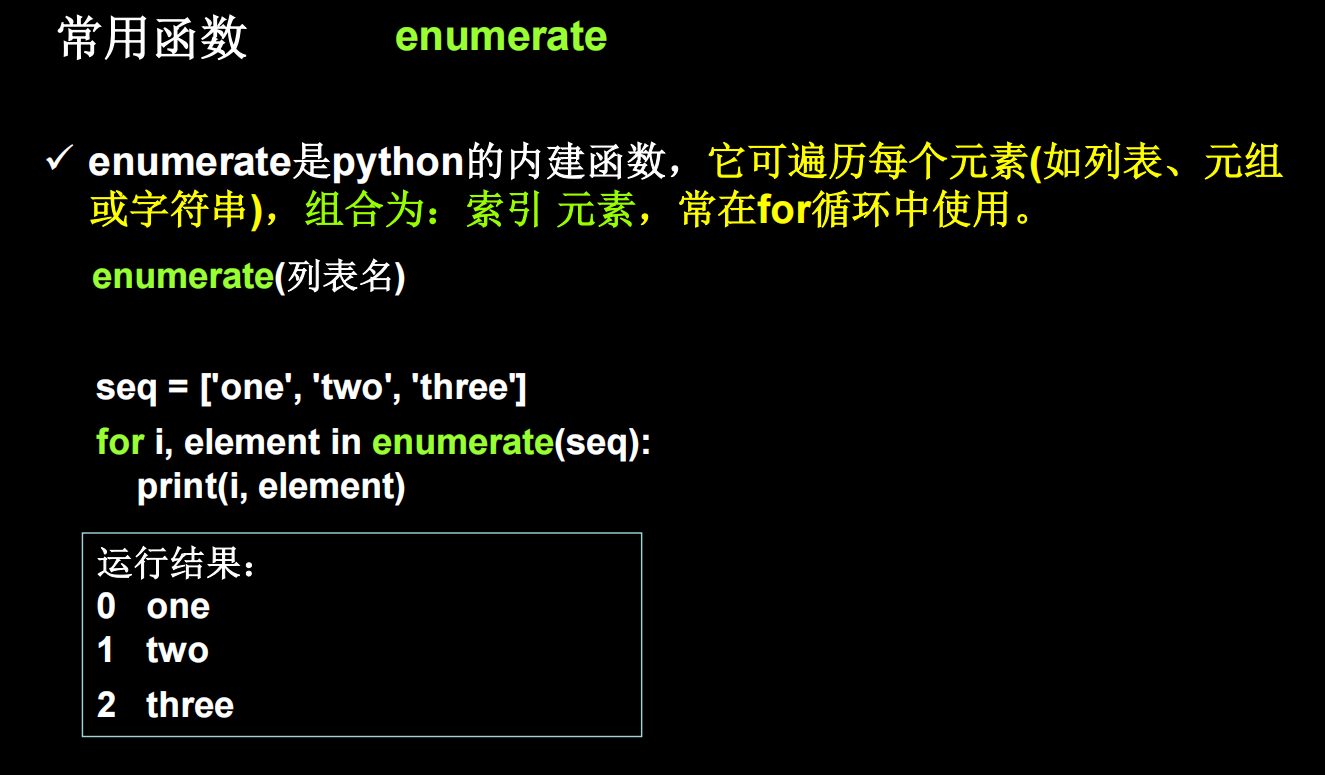
for step, (x_train, y_train) in enumerate(train_db): #batch级别的循环 ,每个step循环一个batch
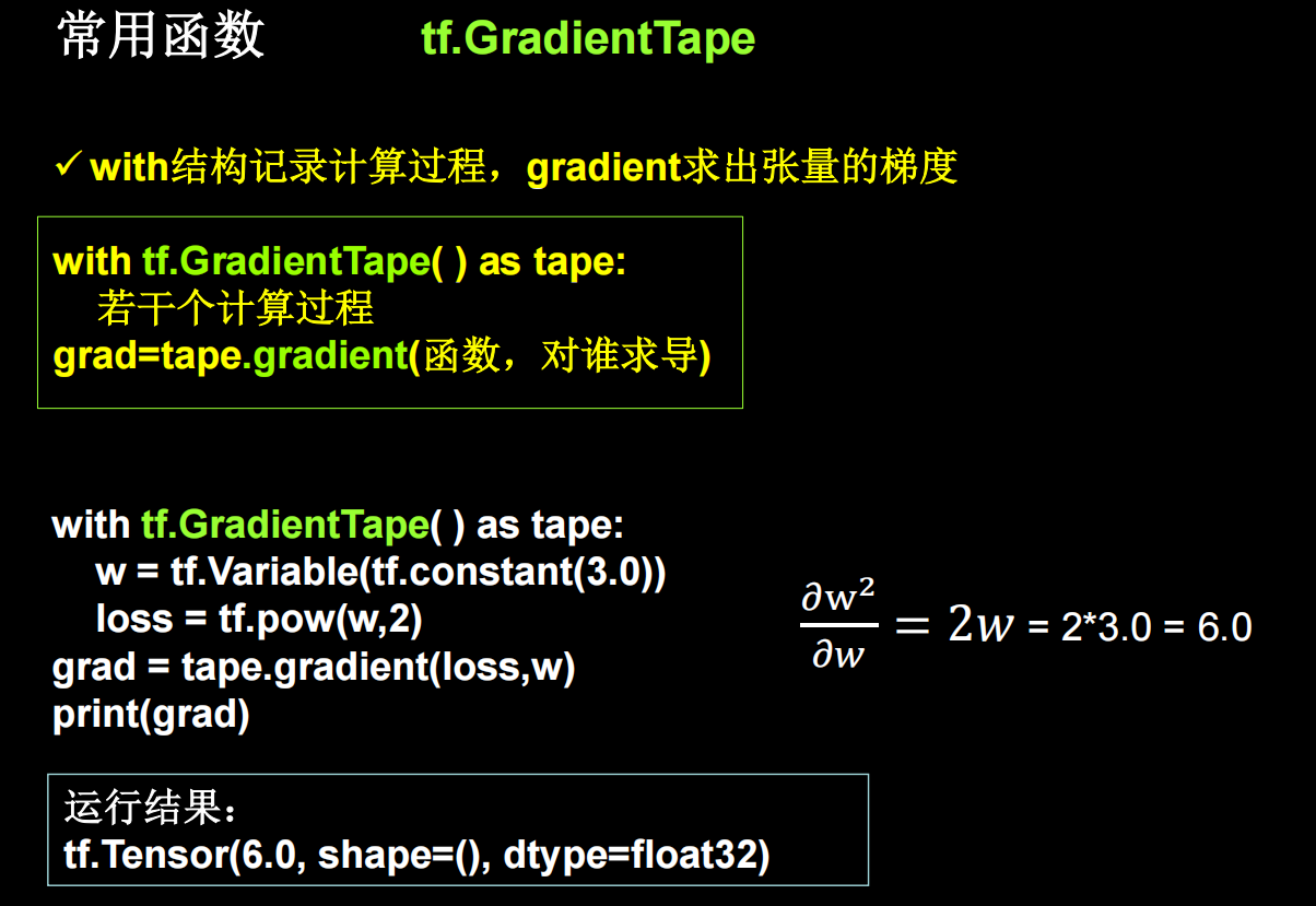
with tf.GradientTape() as tape: # with结构记录梯度信息
y = tf.matmul(x_train, w1) + b1 # 神经网络乘加运算
y = tf.nn.softmax(y) # 使输出y符合概率分布(此操作后与独热码同量级,可相减求loss)
y_ = tf.one_hot(y_train, depth=3) # 将标签值转换为独热码格式,方便计算loss和accuracy
loss = tf.reduce_mean(tf.square(y_ - y)) # 采用均方误差损失函数mse = mean(sum(y-out)^2)
loss_all += loss.numpy() # 将每个step计算出的loss累加,为后续求loss平均值提供数据,这样计算的loss更准确
# 计算loss对各个参数的梯度
grads = tape.gradient(loss, [w1, b1])
# 实现梯度更新 w1 = w1 - lr * w1_grad b = b - lr * b_grad
w1.assign_sub(lr * grads[0]) # 参数w1自更新
b1.assign_sub(lr * grads[1]) # 参数b自更新
# 每个epoch,打印loss信息
print("Epoch {}, loss: {}".format(epoch, loss_all/4))
train_loss_results.append(loss_all / 4) # 将4个step的loss求平均记录在此变量中
loss_all = 0 # loss_all归零,为记录下一个epoch的loss做准备
# 测试部分
# total_correct为预测对的样本个数, total_number为测试的总样本数,将这两个变量都初始化为0
total_correct, total_number = 0, 0
for x_test, y_test in test_db:
# 使用更新后的参数进行预测
y = tf.matmul(x_test, w1) + b1
y = tf.nn.softmax(y)
pred = tf.argmax(y, axis=1) # 返回y中最大值的索引,即预测的分类
# 将pred转换为y_test的数据类型
pred = tf.cast(pred, dtype=y_test.dtype)
# 若分类正确,则correct=1,否则为0,将bool型的结果转换为int型
correct = tf.cast(tf.equal(pred, y_test), dtype=tf.int32)
# 将每个batch的correct数加起来
correct = tf.reduce_sum(correct)
# 将所有batch中的correct数加起来
total_correct += int(correct)
# total_number为测试的总样本数,也就是x_test的行数,shape[0]返回变量的行数
total_number += x_test.shape[0]
# 总的准确率等于total_correct/total_number
acc = total_correct / total_number
test_acc.append(acc)
print("Test_acc:", acc)
print("--------------------------")
# 绘制 loss 曲线
plt.title('Loss Function Curve') # 图片标题
plt.xlabel('Epoch') # x轴变量名称
plt.ylabel('Loss') # y轴变量名称
plt.plot(train_loss_results, label="$Loss$") # 逐点画出trian_loss_results值并连线,连线图标是Loss
plt.legend() # 画出曲线图标
plt.show() # 画出图像
# 绘制 Accuracy 曲线
plt.title('Acc Curve') # 图片标题
plt.xlabel('Epoch') # x轴变量名称
plt.ylabel('Acc') # y轴变量名称
plt.plot(test_acc, label="$Accuracy$") # 逐点画出test_acc值并连线,连线图标是Accuracy
plt.legend()
plt.show()
class2
预备知识
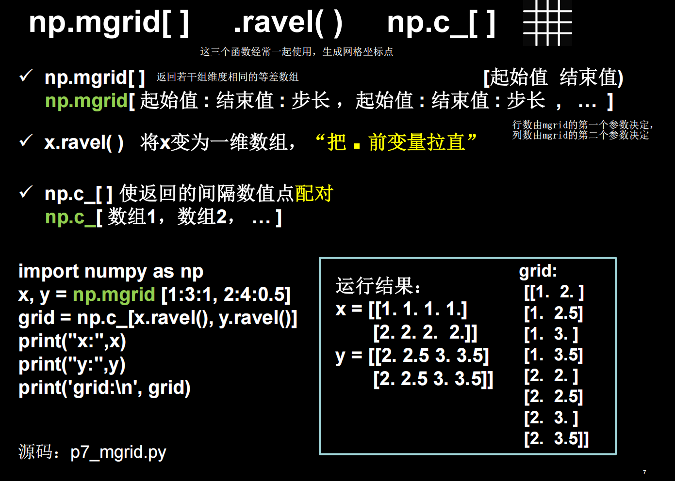
这里,x,y都是二维数组,行数由第一个参数1:3:1决定,为2行,列数由第二个参数2:4:0.5决定,为4列。排布规律为:x跨行方向即列方向与第一个参数一致,y为跨列方向即行方向与第二个参数一致。
使用tensorflow原生代码搭建神经网络
class3
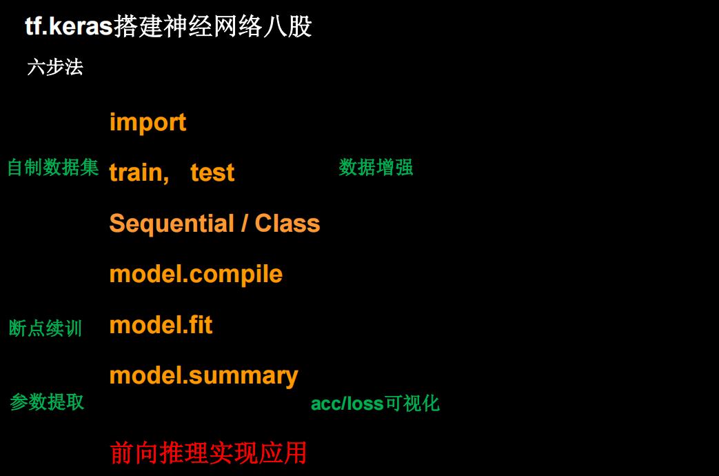
Sequential搭建网络八股
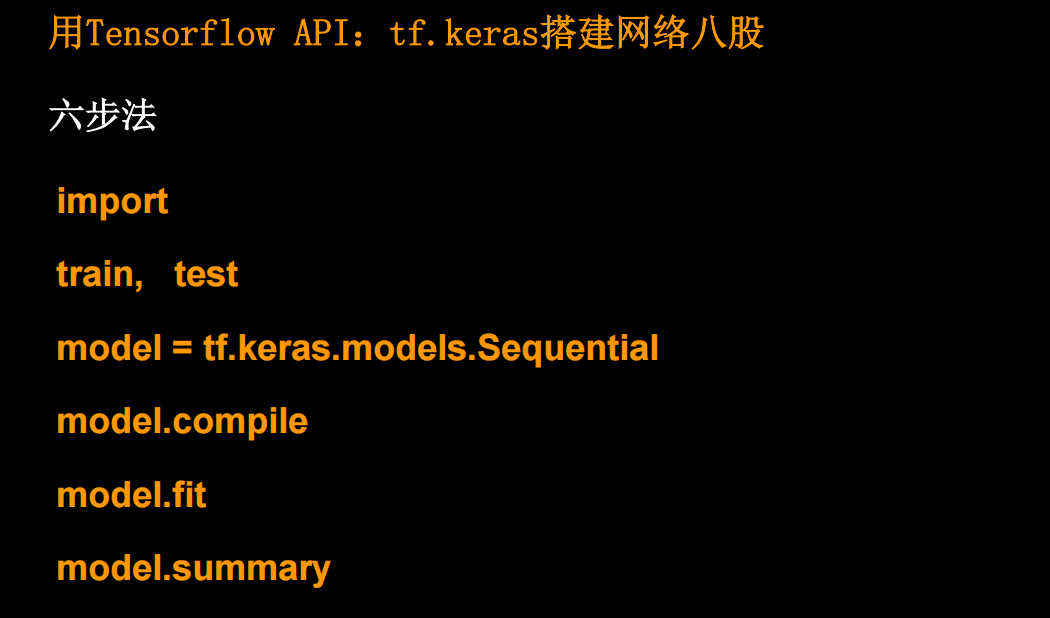
用Tensorflow API:tf.keras搭建网络八股
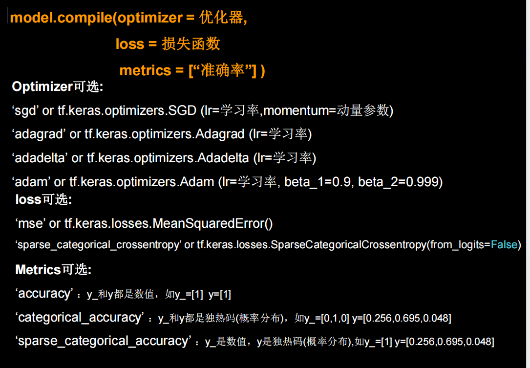
一般选sparse_categorical_accuracy,因为标签是数值,输出是概率分布
loss=tf.keras.losses.SparseCategoricalCrossentropy(from_logits=False)
from_logits=False就是神经网络预测结果输出经过概率分布,如果是结果直接输出,from_logits=True
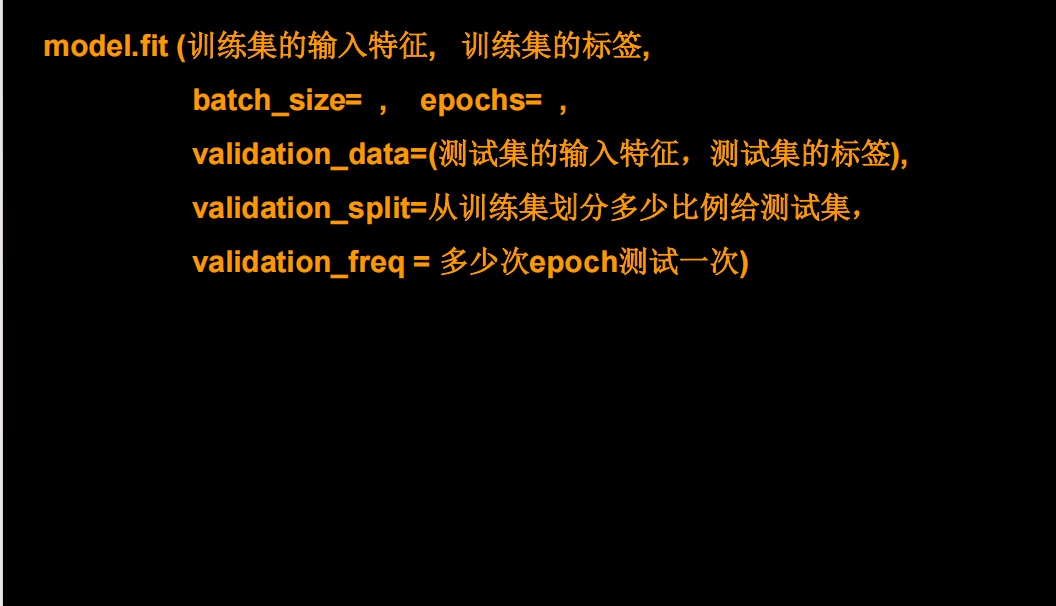
validation data和validation split二者选其中一个就行。下面是一个用keras搭建鸢尾花分类的例子
import tensorflow as tf
from sklearn import datasets
import numpy as np


X = datasets.load_iris().data
Y = datasets.load_iris().target

np.random.seed(13)
np.random.shuffle(X)
np.random.seed(13)
np.random.shuffle(Y)
np.random.seed(13)

model = tf.keras.models.Sequential([tf.keras.layers.Dense(units=3, activation='softmax',
                                                          input_shape=(4,),kernel_regularizer=tf.keras.regularizers.l2())])

model.compile(optimizer=tf.keras.optimizers.Adam(lr=0.1), loss=tf.keras.losses.SparseCategoricalCrossentropy(from_logits=False)
              ,metrics=['sparse_categorical_accuracy'])

model.fit(X,Y,epochs=500,batch_size=32,validation_split=0.2,validation_freq=20)

model.summary()
神经网络中间的隐藏层你可以自己制定,只要保证最后输出层是三个神经元就行,下面中间又加一层也是可行的。
import tensorflow as tf
from sklearn import datasets
import numpy as np


X = datasets.load_iris().data
Y = datasets.load_iris().target

np.random.seed(13)
np.random.shuffle(X)
np.random.seed(13)
np.random.shuffle(Y)
np.random.seed(13)

model = tf.keras.models.Sequential([tf.keras.layers.Dense(units=5, activation='relu',
                                                          input_shape=(4,),kernel_regularizer=tf.keras.regularizers.l2()),
                                    tf.keras.layers.Dense(units=3, activation='softmax',

                                                          kernel_regularizer=tf.keras.regularizers.l2())
                                    ])

model.compile(optimizer=tf.keras.optimizers.Adam(lr=0.1), loss=tf.keras.losses.SparseCategoricalCrossentropy(from_logits=False)
              ,metrics=['sparse_categorical_accuracy'])

model.fit(X,Y,epochs=500,batch_size=32,validation_split=0.2,validation_freq=20)

model.summary()
用类搭建网络八股
Sequential可以搭建上层输出就是下层输入的顺序网络结构,但是无法写出一些带有跳连的非顺序网络结构。这时候可以使用类MyModel封装一个网络结构
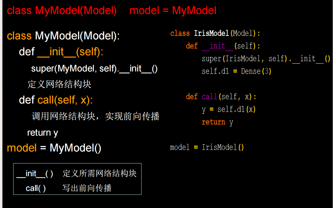
self.d1,d1是这一层的名字
import tensorflow as tf
import numpy as np
from sklearn import datasets
from tensorflow.keras import Model
from tensorflow.keras.layers import Dense, Dropout

x_train=datasets.load_iris().data
y_train=datasets.load_iris().target

np.random.seed(33)
np.random.shuffle(x_train)
np.random.seed(33)
np.random.shuffle(y_train)
np.random.seed(33)


class IrisModel(Model):
    def __init__(self):
        super(IrisModel, self).__init__()
        self.d1=tf.keras.layers.Dense(3, activation='softmax',)

    def call(self,x):
        y=self.d1(x)
        return y


model=IrisModel()
model.compile(optimizer=tf.keras.optimizers.SGD(lr=0.1),
              loss=tf.keras.losses.SparseCategoricalCrossentropy(from_logits=False),
              metrics=['sparse_categorical_accuracy'])
model.fit(x_train,y_train,batch_size=32,epochs=500,validation_split=0.3,validation_freq=50)
model.summary()
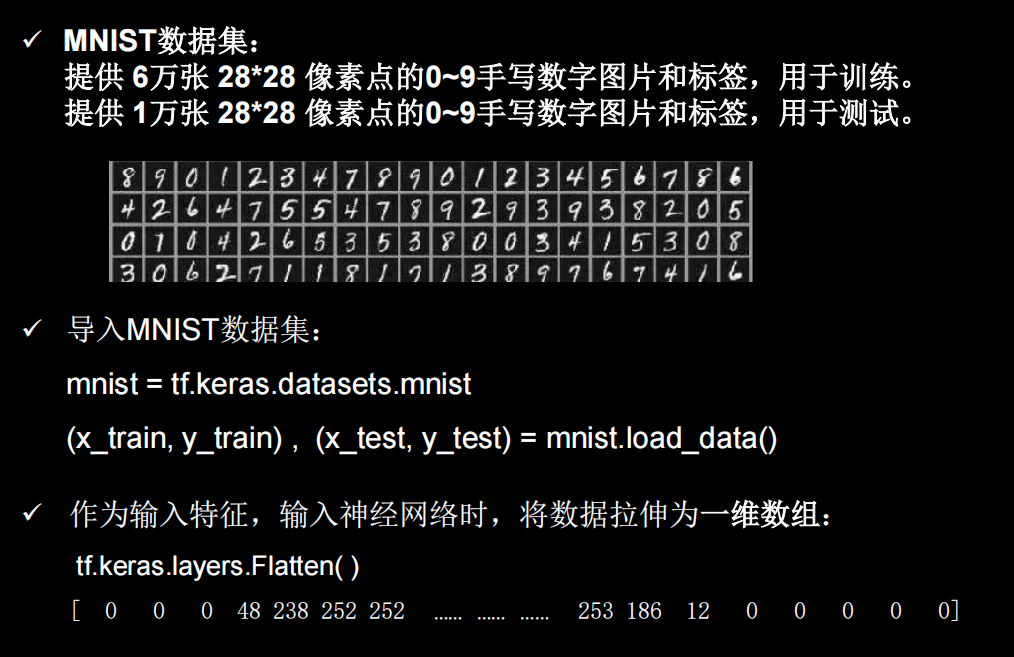
MINIST数据集
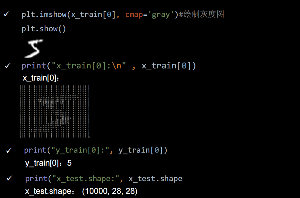
可视化数据
import tensorflow as tf
from matplotlib import pyplot as plt

mnist = tf.keras.datasets.mnist
(x_train, y_train), (x_test, y_test) = mnist.load_data()

# 可视化训练集输入特征的第一个元素
plt.imshow(x_train[0], cmap='gray')  # 绘制灰度图
plt.show()

# 打印出训练集输入特征的第一个元素
print("x_train[0]:\n", x_train[0])
# 打印出训练集标签的第一个元素
print("y_train[0]:\n", y_train[0])

# 打印出整个训练集输入特征形状
print("x_train.shape:\n", x_train.shape)
# 打印出整个训练集标签的形状
print("y_train.shape:\n", y_train.shape)
# 打印出整个测试集输入特征的形状
print("x_test.shape:\n", x_test.shape)
# 打印出整个测试集标签的形状
print("y_test.shape:\n", y_test.shape)
训练模型
import tensorflow as tf
from tensorflow.keras import datasets, layers, models


(x_train, y_train), (x_test, y_test) = datasets.mnist.load_data()
x_train, x_test = x_train / 255.0, x_test / 255.0
model=tf.keras.models.Sequential([
    layers.Flatten(),
    layers.Dense(128, activation='relu'),
    layers.Dense(10, activation='softmax')
])
model.compile(optimizer=tf.keras.optimizers.Adam(lr=0.01),
              loss=tf.keras.losses.SparseCategoricalCrossentropy(from_logits=False),
              metrics=['sparse_categorical_accuracy'])

model.fit(x_train,y_train,epochs=5, batch_size=128, validation_data=(x_test,y_test),
          validation_freq=1)

model.summary()
因为最后一层激活函数是softmax,输出已经符合概率分布,所以loss中的参数from_logits=False。如果最后一层激活函数是relu,from_logits=True
import tensorflow as tf
from tensorflow.keras import datasets, layers, models


(x_train, y_train), (x_test, y_test) = datasets.mnist.load_data()
x_train, x_test = x_train / 255.0, x_test / 255.0
model=tf.keras.models.Sequential([
    layers.Flatten(),
    layers.Dense(128, activation='relu'),
    layers.Dense(10, activation='relu')
])
model.compile(optimizer=tf.keras.optimizers.Adam(lr=0.01),
              loss=tf.keras.losses.SparseCategoricalCrossentropy(from_logits=True),
              metrics=['sparse_categorical_accuracy'])

model.fit(x_train,y_train,epochs=5, batch_size=128, validation_data=(x_test,y_test),
          validation_freq=1)

model.summary()
用类函数实现
import tensorflow as tf
from tensorflow.keras import layers,datasets,Model

(x_train, y_train), (x_test, y_test) = datasets.mnist.load_data()
x_train, x_test = x_train / 255.0, x_test/255.0

class MinistModel(Model):
    def __init__(self):
        super(MinistModel, self).__init__()
        self.fc1 = layers.Flatten()
        self.fc2 = layers.Dense(128, activation='relu')
        self.fc3 = layers.Dense(10, activation='softmax')

    def call(self,x):
        x = self.fc1(x)
        x = self.fc2(x)
        x = self.fc3(x)
        return x

model = MinistModel()
model.compile(optimizer='adam',loss='sparse_categorical_crossentropy',
              metrics=['sparse_categorical_accuracy'])
model.fit(x_train, y_train, epochs=5, batch_size=128,validation_data=(x_test, y_test),validation_freq=1)
model.summary()
FASHION数据集

用Sequential实现
import tensorflow as tf
from tensorflow.keras import datasets, layers
from tensorflow.keras import Model

(x_train, y_train), (x_test, y_test) = tf.keras.datasets.fashion_mnist.load_data()
x_train, x_test = x_train / 255.0, x_test/255.0

model = tf.keras.models.Sequential([
    layers.Flatten(),
    layers.Dense(128,activation='relu'),
    layers.Dense(10, activation='relu')
])
model.compile(optimizer='adam', loss=tf.keras.losses.SparseCategoricalCrossentropy(from_logits=True)
              , metrics=['sparse_categorical_accuracy'])
model.fit(x_train, y_train, epochs=5, batch_size=128, validation_data=(x_test, y_test),validation_freq=1)
model.summary()
用类实现
import tensorflow as tf
from tensorflow.keras import layers, Model

class FashionMNIST(Model):
    def __init__(self):
        super(FashionMNIST, self).__init__()
        self.layer1 = layers.Flatten()
        self.layer2 = layers.Dense(128, activation='relu')
        self.layer3 = layers.Dense(10, activation='softmax')

    def call(self, x):
        x = self.layer1(x)
        x = self.layer2(x)
        x = self.layer3(x)
        return x


(x_train, y_train), (x_test, y_test) = tf.keras.datasets.fashion_mnist.load_data()
x_train, x_test = x_train / 255.0, x_test/255.0

model = FashionMNIST()
model.compile(optimizer='adam', loss=tf.keras.losses.SparseCategoricalCrossentropy(from_logits=True),
              metrics=['sparse_categorical_accuracy'])
model.fit(x_train, y_train, batch_size=128, epochs=5, validation_data=(x_test, y_test),validation_freq=1)
model.summary()
class4
自制数据集
数据集下载提取码:mocm
之前都是进行的训练都是tensorflow自带的数据集,这些数据集特征表现好,因此容易训练出好的效果。如果要训练自己的数据集该怎么做
这一讲将进行扩充

回想一下之前的代码class3.3中数据的读入
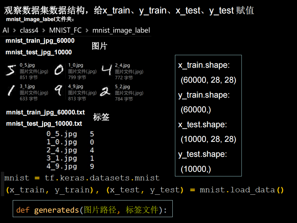
先写一个读取数据的函数generateds
import numpy as np
import tensorflow as tf
import os
from PIL import Image

def generateds(path,txt):
    f=open(txt,'r')
    contexts=f.readlines()
    f.close()  # 别忘了,不然Too many open files
    x,y_=[],[]
    for context in contexts:
        values=context.split()
        img_path=path+'\\'+values[0]
        img=Image.open(img_path)
        img = np.array(img.convert('L'))   # 别忘了转换图片格式
        img = img / 255.
        x.append(img)
        y_.append(values[1])
        # print(type(values[1]))
        print('loading : ' + context)

    x=np.array(x)
    y_=np.array(y_)
    y_=y_.astype(np.int64)     # 把str转换成int
    return x,y_

if __name__=='__main__':
    path=r'D:\code\python\TF2.0\class4\MNIST_FC\mnist_image_label\mnist_train_jpg_60000'
    txt=r'D:\code\python\TF2.0\class4\MNIST_FC\mnist_image_label\mnist_train_jpg_60000.txt'
    x,y=generateds(path,txt)
    print(x.shape)
    print(y.shape)
然后把之前训练的步骤加上
import numpy as np
import tensorflow as tf
import os
from PIL import Image
from tensorflow import keras

def generateds(path,txt):
    f=open(txt,'r')
    contexts=f.readlines()
    f.close()  # 别忘了,不然Too many open files
    x,y_=[],[]
    for context in contexts:
        values=context.split()
        img_path=path+'\\'+values[0]
        img=Image.open(img_path)
        img = np.array(img.convert('L'))   # 别忘了转换图片格式
        img = img / 255.
        x.append(img)
        y_.append(values[1])
        # print(type(values[1]))
        print('loading : ' + context)

    x=np.array(x)
    y_=np.array(y_)
    y_=y_.astype(np.int64)     # 把str转换成int
    return x,y_

if __name__=='__main__':
    train_path=r'D:\code\python\TF2.0\class4\MNIST_FC\mnist_image_label\mnist_train_jpg_60000'
    train_label=r'D:\code\python\TF2.0\class4\MNIST_FC\mnist_image_label\mnist_train_jpg_60000.txt'
    train_save_path=r'D:\code\python\TF2.0\class4\MNIST_FC\mnist_image_label\mnist_x_train.npy'
    train_label_save_path=r'D:\code\python\TF2.0\class4\MNIST_FC\mnist_image_label\mnist_y_train.npy'

    test_path=r'D:\code\python\TF2.0\class4\MNIST_FC\mnist_image_label\mnist_test_jpg_10000'
    test_label=r'D:\code\python\TF2.0\class4\MNIST_FC\mnist_image_label\mnist_test_jpg_10000.txt'
    test_save_path=r'D:\code\python\TF2.0\class4\MNIST_FC\mnist_image_label\mnist_x_test.npy'
    test_label_save_path = r'D:\code\python\TF2.0\class4\MNIST_FC\mnist_image_label\mnist_y_test.npy'

    if os.path.exists(train_save_path) and os.path.exists(train_label_save_path) and os.path.exists(
            test_save_path) and os.path.exists(test_label_save_path):
        print('-------------Load Datasets-----------------')
        x_train=np.load(train_save_path)
        print(x_train.shape)
        y_train=np.load(train_label_save_path)
        print(y_train.shape)
        x_test=np.load(test_save_path)
        print(x_test.shape)
        y_test=np.load(test_label_save_path)
        print(y_test.shape)
    else:
        print('-------------Generate Datasets-----------------')
        x_train,y_train=generateds(train_path,train_label)
        x_test,y_test=generateds(test_path,test_label)
        print('-------------Save Datasets-----------------')

        np.save(train_save_path,x_train)
        np.save(train_label_save_path,y_train)
        np.save(test_save_path,x_test)
        np.save(test_label_save_path,y_test)


    model=tf.keras.models.Sequential([
        tf.keras.layers.Flatten(),
        tf.keras.layers.Dense(512, activation='relu'),
        tf.keras.layers.Dense(10, activation='softmax')
    ])

    model.compile(optimizer='adam',loss=tf.keras.losses.SparseCategoricalCrossentropy(from_logits=False),
                  metrics=['sparse_categorical_accuracy'])
    model.fit(x_train,y_train,epochs=5,validation_data=(x_test,y_test),batch_size=32,validation_freq=1)
    model.summary()
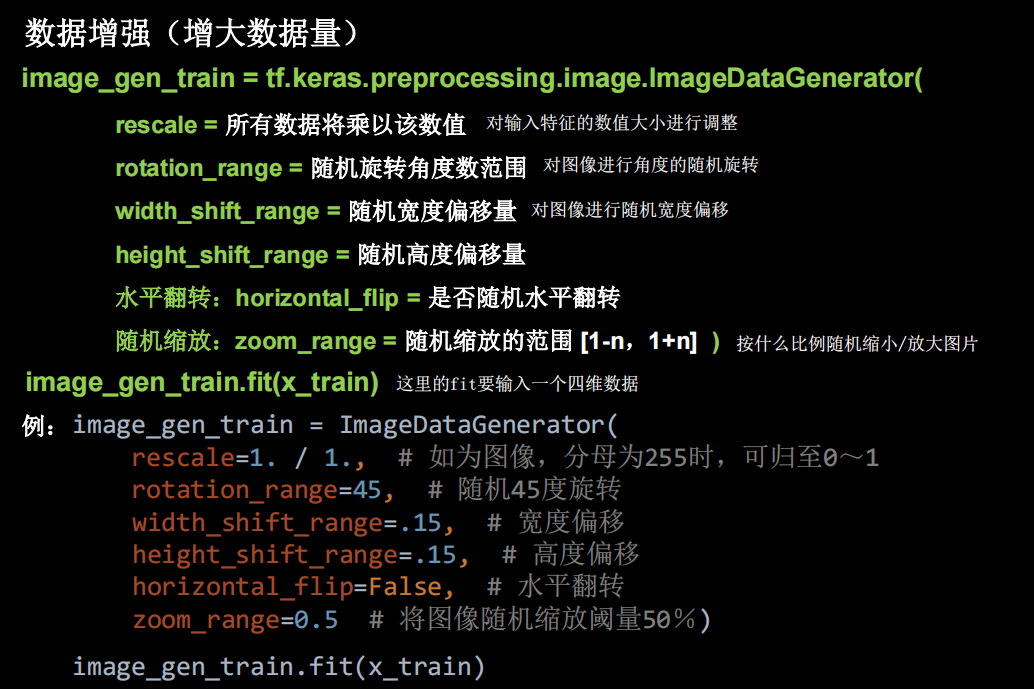
数据增强
import tensorflow as tf
from tensorflow.keras import datasets, layers
from tensorflow.keras import Model
from tensorflow.keras.preprocessing.image import ImageDataGenerator


image_gen_train=ImageDataGenerator(
                        rescale =1./1.,
                        rotation_range = 45,
                        width_shift_range =.15 ,
                        height_shift_range =.15,
                        horizontal_flip =False,
                        zoom_range =0.5 )

(x_train, y_train), (x_test, y_test) = tf.keras.datasets.mnist.load_data()
x_train, x_test = x_train / 255.0, x_test/255.0
x_train = x_train.reshape(x_train.shape[0],28,28,1)
image_gen_train.fit(x_train)

model = tf.keras.models.Sequential([
    layers.Flatten(),
    layers.Dense(128,activation='relu'),
    layers.Dense(10, activation='relu')
])
model.compile(optimizer='adam', loss=tf.keras.losses.SparseCategoricalCrossentropy(from_logits=True)
               ,metrics=['sparse_categorical_accuracy'])
model.fit(image_gen_train.flow(x_train,y_train,batch_size=32), epochs=5, validation_data=(x_test, y_test)
          ,validation_freq=1)
model.summary()
数据增强在小数据上能增加模型泛化效果
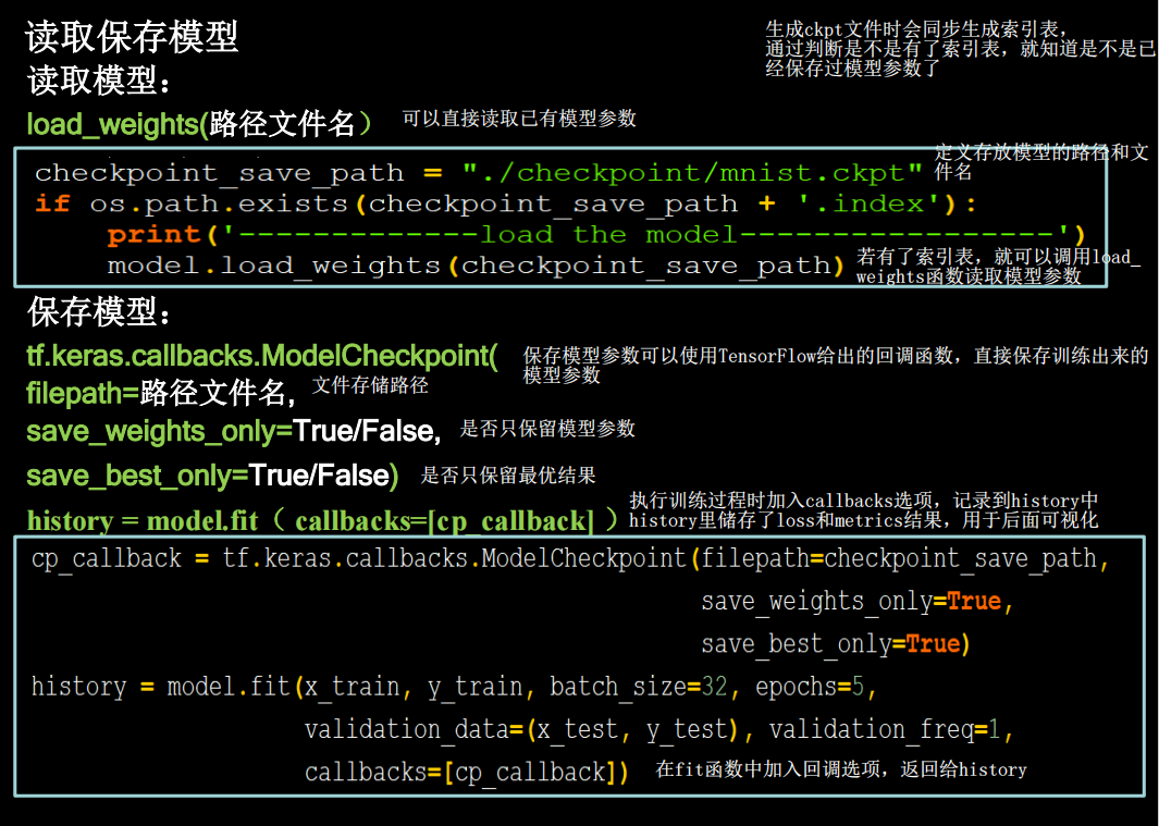
断点续训
import tensorflow as tf
from tensorflow.keras import datasets, layers
from tensorflow.keras import Model
from tensorflow.keras.preprocessing.image import ImageDataGenerator
import os
(x_train, y_train), (x_test, y_test) = tf.keras.datasets.mnist.load_data()
x_train, x_test = x_train / 255.0, x_test/255.0
x_train = x_train.reshape(x_train.shape[0],28,28,1)
model = tf.keras.models.Sequential([
layers.Flatten(),
layers.Dense(128,activation='relu'),
layers.Dense(10, activation='relu')
])
model.compile(optimizer='adam', loss=tf.keras.losses.SparseCategoricalCrossentropy(from_logits=True)
,metrics=['sparse_categorical_accuracy'])
checkpoint_save_path="./checkpoints/mnist.ckpt"
if os.path.exists(checkpoint_save_path+'.index'):
model.load_weights(checkpoint_save_path)
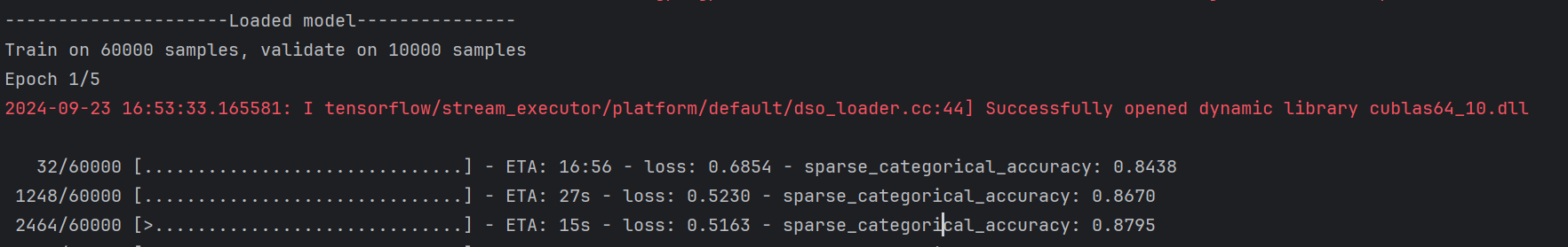
print("---------------------Loaded model---------------")
cp_callback = tf.keras.callbacks.ModelCheckpoint(filepath=checkpoint_save_path, save_weights_only=True
,save_best_only=True)
history=model.fit(x_train,y_train,batch_size=32, epochs=5, validation_data=(x_test, y_test)
,validation_freq=1,callbacks=[cp_callback])
model.summary()
会发现加载了之前的模型,并接着训练
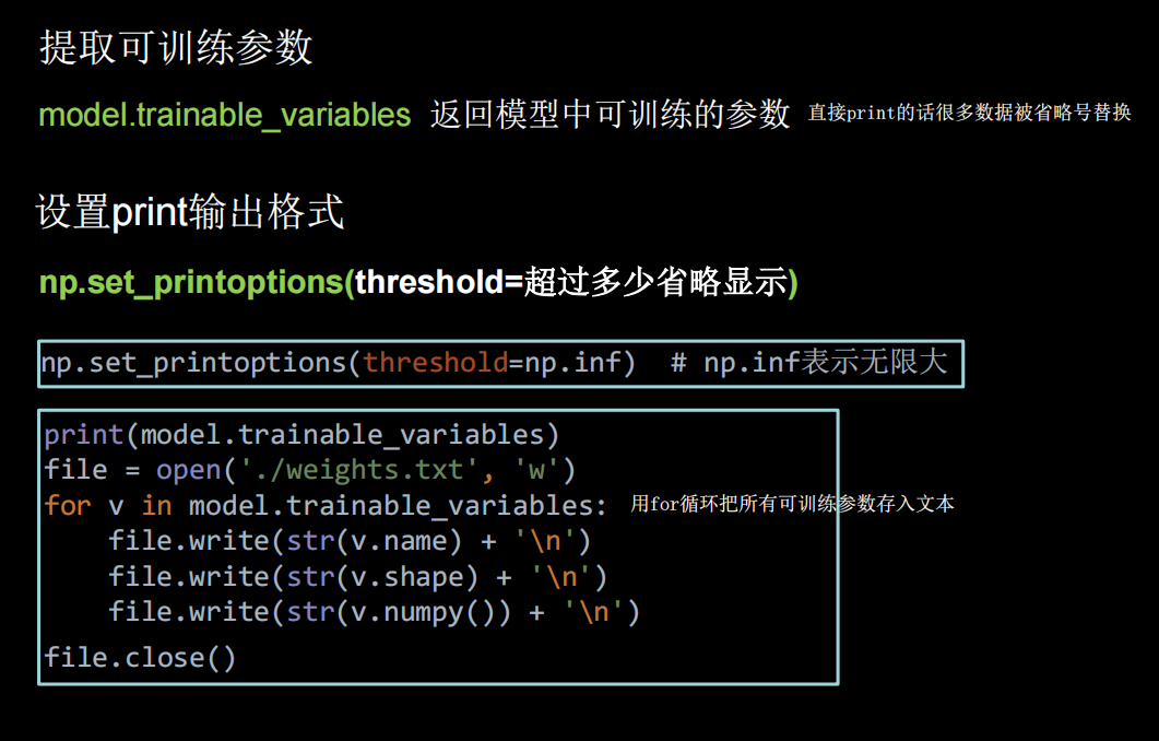
参数提取
import tensorflow as tf
from tensorflow.keras import datasets, layers
from tensorflow.keras import Model
from tensorflow.keras.preprocessing.image import ImageDataGenerator
import os
import numpy as np
np.set_printoptions(threshold=np.inf)


(x_train, y_train), (x_test, y_test) = tf.keras.datasets.mnist.load_data()
x_train, x_test = x_train / 255.0, x_test/255.0
x_train = x_train.reshape(x_train.shape[0],28,28,1)


model = tf.keras.models.Sequential([
    layers.Flatten(),
    layers.Dense(128,activation='relu'),
    layers.Dense(10, activation='relu')
])
model.compile(optimizer='adam', loss=tf.keras.losses.SparseCategoricalCrossentropy(from_logits=True)
               ,metrics=['sparse_categorical_accuracy'])

checkpoint_save_path="./checkpoints/mnist.ckpt"
if os.path.exists(checkpoint_save_path+'.index'):
    model.load_weights(checkpoint_save_path)
    print("---------------------Loaded model---------------")

cp_callback = tf.keras.callbacks.ModelCheckpoint(filepath=checkpoint_save_path, save_weights_only=True
                                              ,save_best_only=True)


history=model.fit(x_train,y_train,batch_size=32, epochs=5, validation_data=(x_test, y_test)
          ,validation_freq=1,callbacks=[cp_callback])
model.summary()
print(model.trainable_variables)
file=open('weights.txt','w')
for v in model.trainable_variables:
    file.write(str(v.name)+'\n')
    file.write(str(v.shape)+'\n')
    file.write(str(v.numpy())+'\n')
file.close()
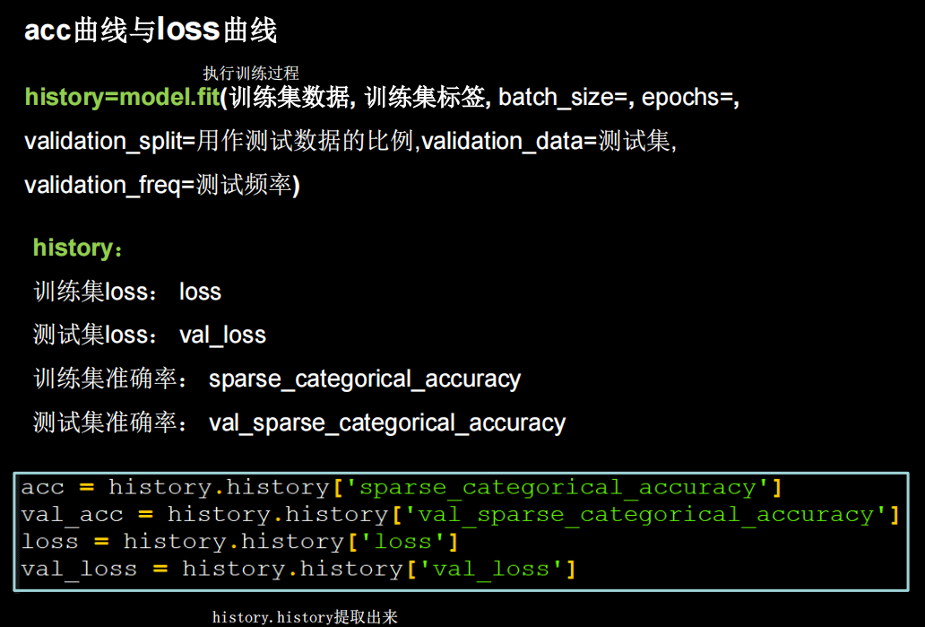
acc&loss可视化
import matplotlib.pyplot as plt
import tensorflow as tf
from tensorflow.keras import datasets, layers
from tensorflow.keras import Model
from tensorflow.keras.preprocessing.image import ImageDataGenerator
import os
import numpy as np
np.set_printoptions(threshold=np.inf)


(x_train, y_train), (x_test, y_test) = tf.keras.datasets.mnist.load_data()
x_train, x_test = x_train / 255.0, x_test/255.0
x_train = x_train.reshape(x_train.shape[0],28,28,1)


model = tf.keras.models.Sequential([
    layers.Flatten(),
    layers.Dense(128,activation='relu'),
    layers.Dense(10, activation='softmax')
])
model.compile(optimizer='adam', loss=tf.keras.losses.SparseCategoricalCrossentropy(from_logits=False)
               ,metrics=['sparse_categorical_accuracy'])

checkpoint_save_path="./checkpoints/mnist.ckpt"
if os.path.exists(checkpoint_save_path+'.index'):
    model.load_weights(checkpoint_save_path)
    print("---------------------Loaded model---------------")

cp_callback = tf.keras.callbacks.ModelCheckpoint(filepath=checkpoint_save_path, save_weights_only=True
                                              ,save_best_only=True)


history=model.fit(x_train,y_train,batch_size=32, epochs=5, validation_data=(x_test, y_test)
          ,validation_freq=1,callbacks=[cp_callback])
model.summary()
print(model.trainable_variables)
file=open('weights.txt','w')
for v in model.trainable_variables:
    file.write(str(v.name)+'\n')
    file.write(str(v.shape)+'\n')
    file.write(str(v.numpy())+'\n')
file.close()
# 绘图
acc=history.history['sparse_categorical_accuracy']
val_acc=history.history['val_sparse_categorical_accuracy']
loss=history.history['loss']
val_loss=history.history['val_loss']

plt.subplot(1,2,1)
plt.plot(acc,label='train acc')
plt.plot(val_acc,label='validation acc')
plt.title('Training and validation accuracy')
plt.legend()

plt.subplot(1,2,2)
plt.plot(loss,label='train loss')
plt.plot(val_loss,label='val loss')
plt.title('Training and validation loss')
plt.legend()
plt.show()
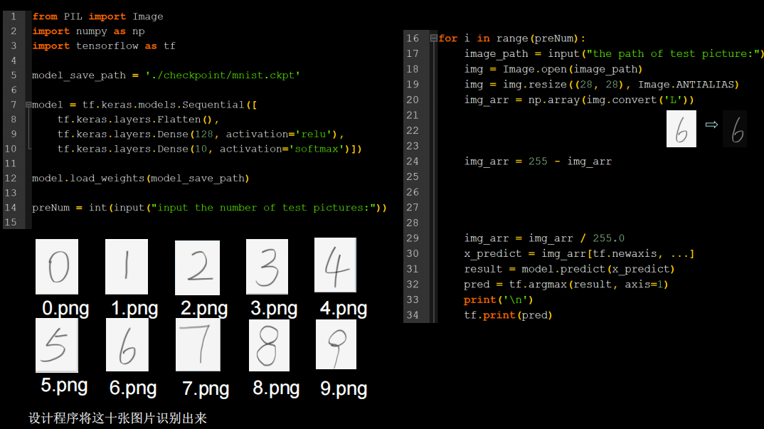
应用程序,给图识物

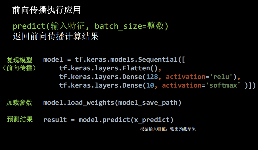
程序
img_arr=img_arr/255.0
是因为训练数据是黑底白字,而预测的数据是白底黑字,需要进行数据预处理,使输入数据满足训练数据特征
for i in range(28):
    for j in range(28):
        if img_arr[i][j] < 200:
            img_arr[i][j] = 255
        else:
            img_arr[i][j] = 0
上面代码可以让输入输出图片变成只有黑白的高对比图像
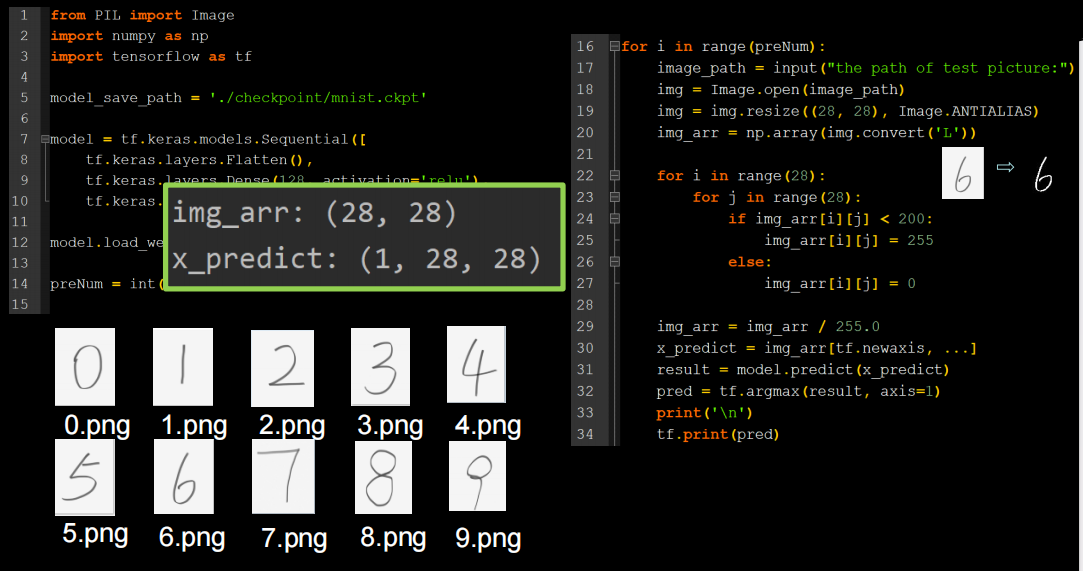
x_predict = img_arr[tf.newaxis, ...]
因为神经网络输入都是一个batch一个batch的输入,所以要增加一个维度。
import os

from PIL import Image
import numpy as np
import tensorflow as tf
from matplotlib import pyplot as plt

model_path=r'D:\code\python\TF2.0\checkpoints\mnist.ckpt'
model = tf.keras.models.Sequential([
    tf.keras.layers.Flatten(),
    tf.keras.layers.Dense(128, activation='relu'),
    tf.keras.layers.Dense(10, activation='softmax')])

model.load_weights(model_path)


x_test_path=r'D:\code\python\TF2.0\class4\MNIST_FC\test'
path=os.listdir(x_test_path)
for img_path in path:
    img_path_=os.path.join(x_test_path,img_path)
    img = Image.open(img_path_)

    img=img.resize((28,28),Image.ANTIALIAS)
    img_arr=np.array(img.convert('L'))


    for i in range(28):
        for j in range(28):
            if img_arr[i][j] < 200:
                img_arr[i][j] = 255
            else:
                img_arr[i][j] = 0

    img_arr = img_arr / 255.0
    x_pred=img_arr[tf.newaxis,...]
    prediction=model.predict(x_pred)

    pre=tf.argmax(prediction,axis=1)
    print('\n')
    tf.print(pre)
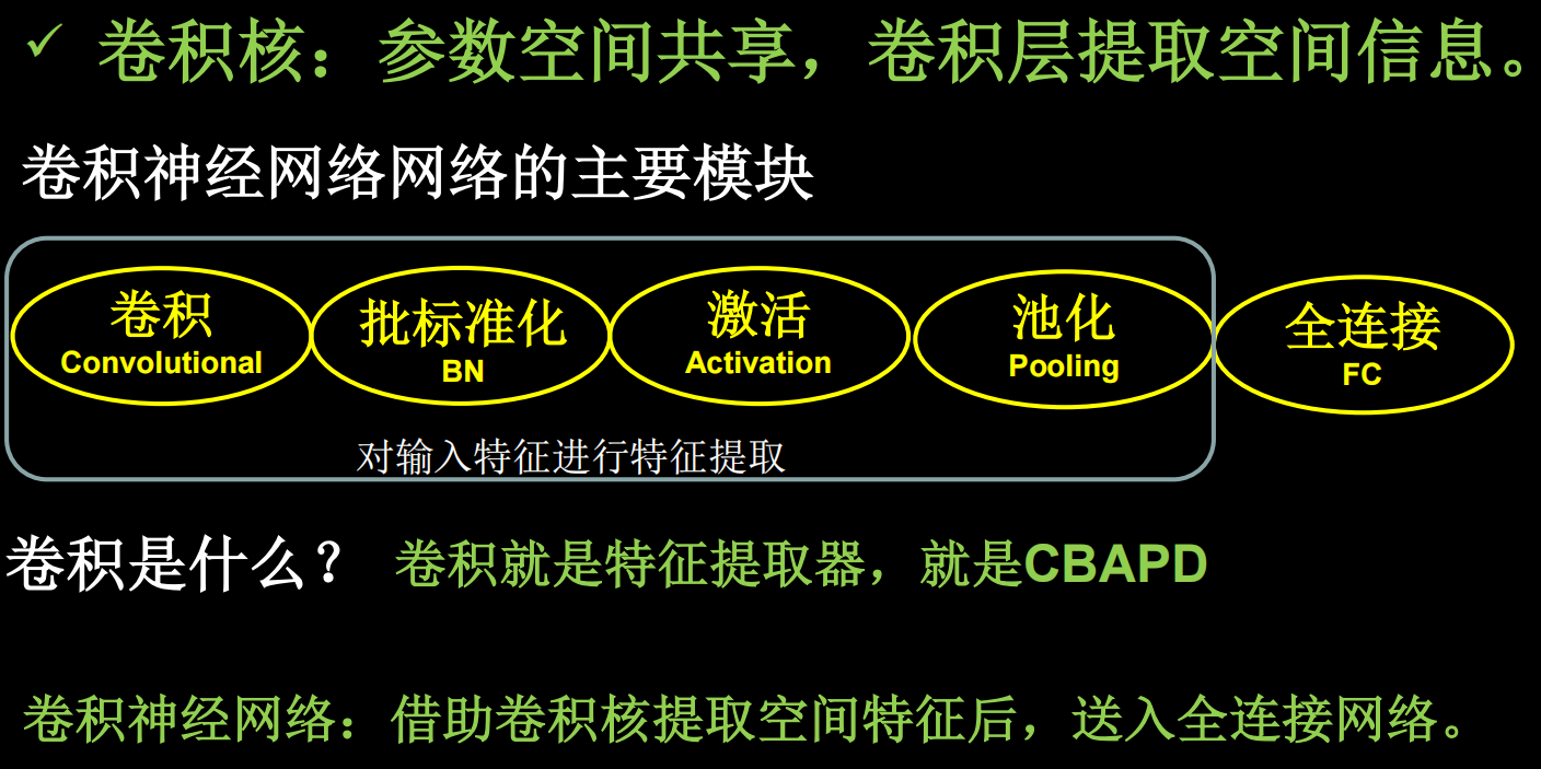
class5
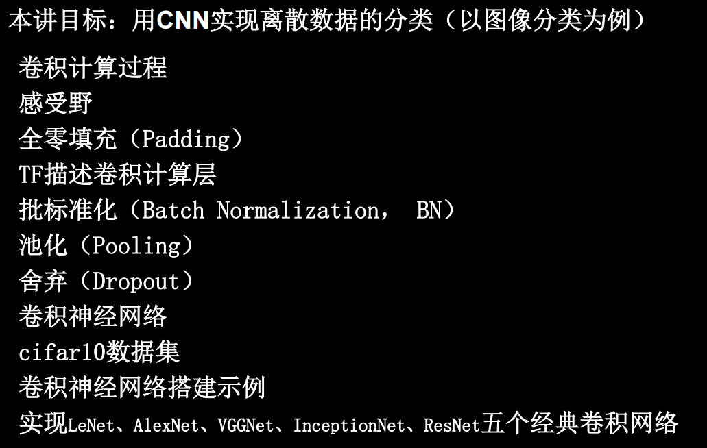
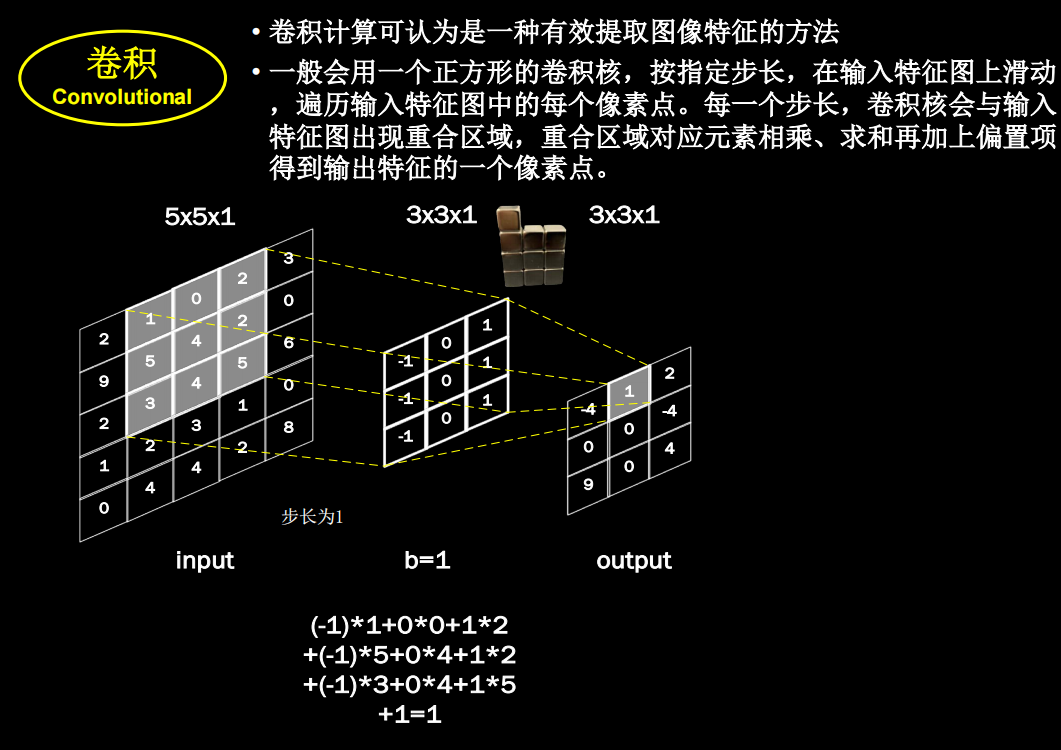
卷积计算过程
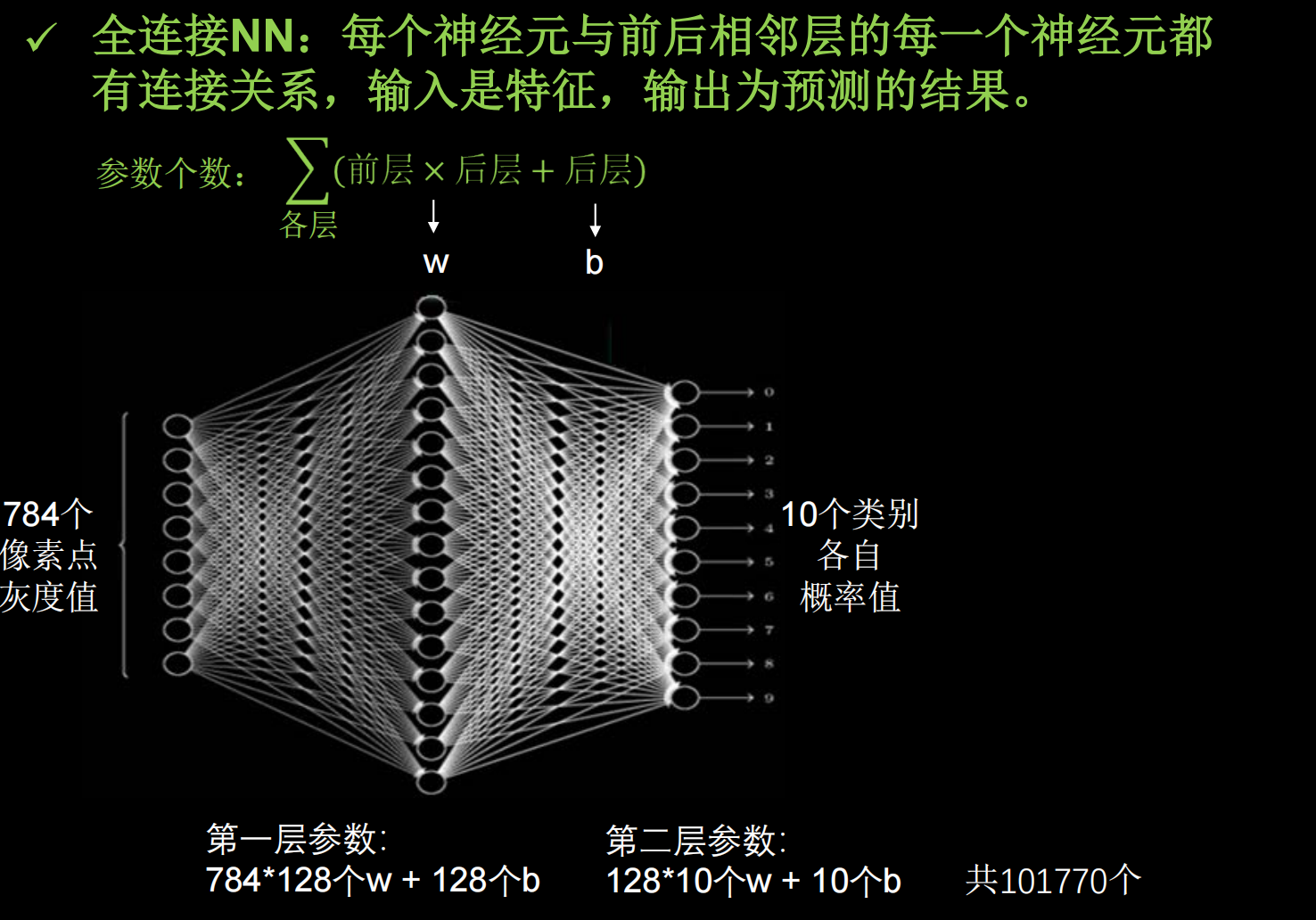
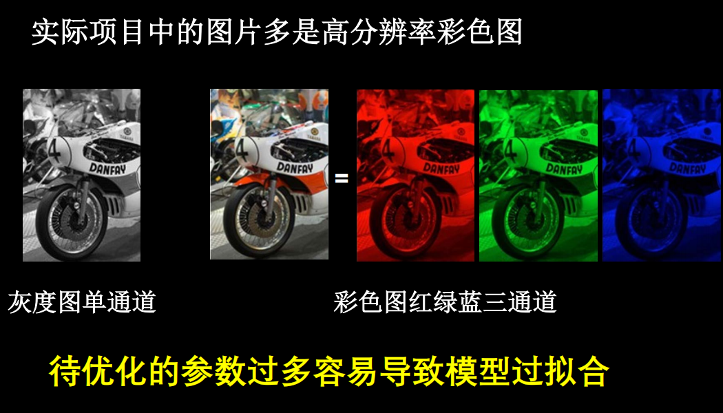
然而实际图像一般是三通道,参数会更多
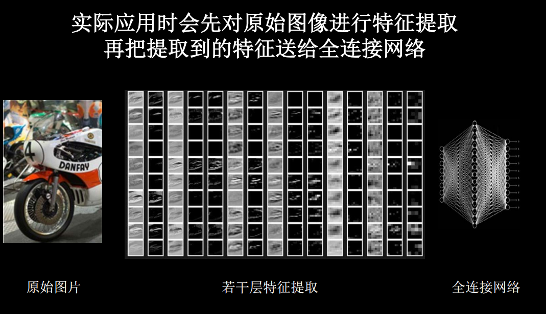
先用cov进行特征提取再进行全连接(yolo中甚至直接不用全连接,只用cov)

卷积核的channel和输入特征图的channel要保持一致
输入是三通道时


具体的计算过程
对于输入特征图是三通道的
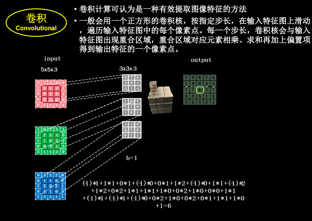
下面看一个动图,会更好的理解

感受野
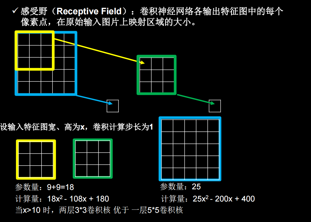
经过两个3×3的卷积和经过一个5×5的卷积的区别是什么?当x也就是图像边长大于10的时候,两个3×3的卷积比一个5×5的卷积效果要好
全零填充
如果希望卷积后输入特征的尺寸不变,就可以输入特征图进行全0填充
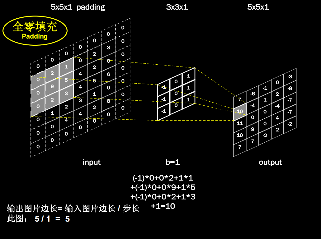
计算公式
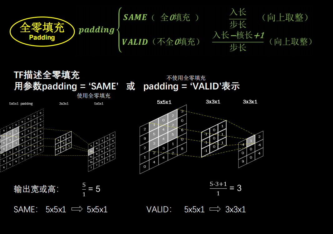
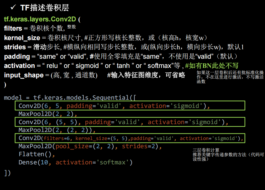
TF描述卷积层
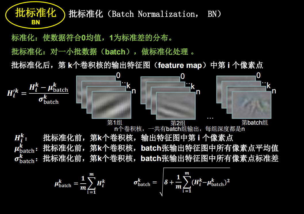
批标准化
神经网络对零均值的数据拟合更好,但是随着神经网络层数的增加,数据还会偏离0均值,用标准化可以把数据拉回来。一般用在卷积和激活函数之间。
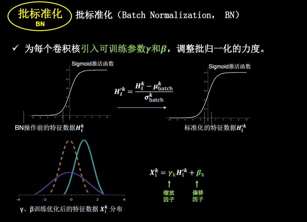
但是如果只进行上面这种简单的标准化,数据都分布在sigmoid函数中间的线性部分,失去了非线性化,因此又引入了两个训练参数,保证了网络的非线性表达力
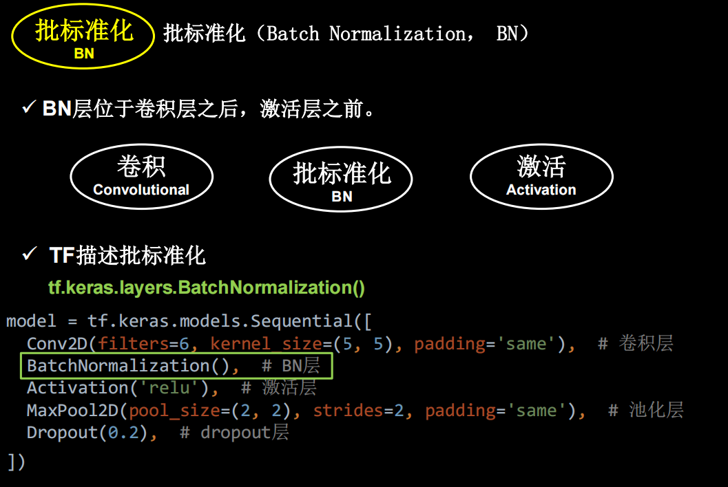
tensorflow中是
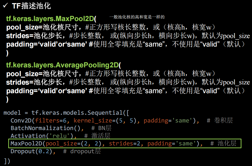
池化
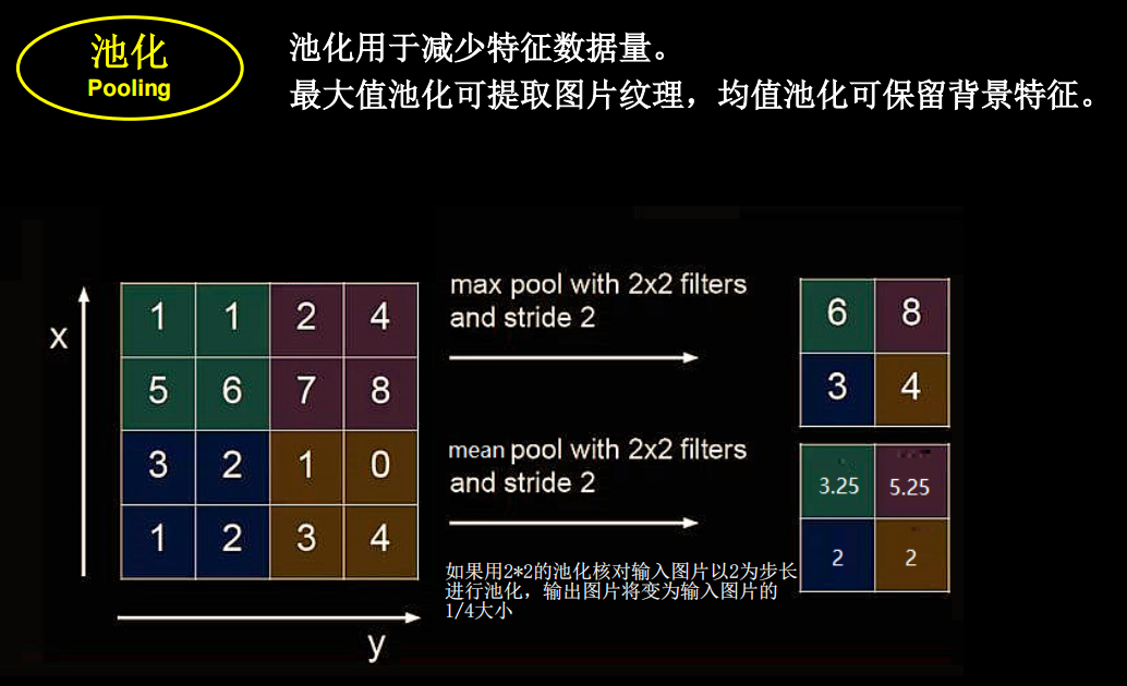
tf中的池化函数
dropout
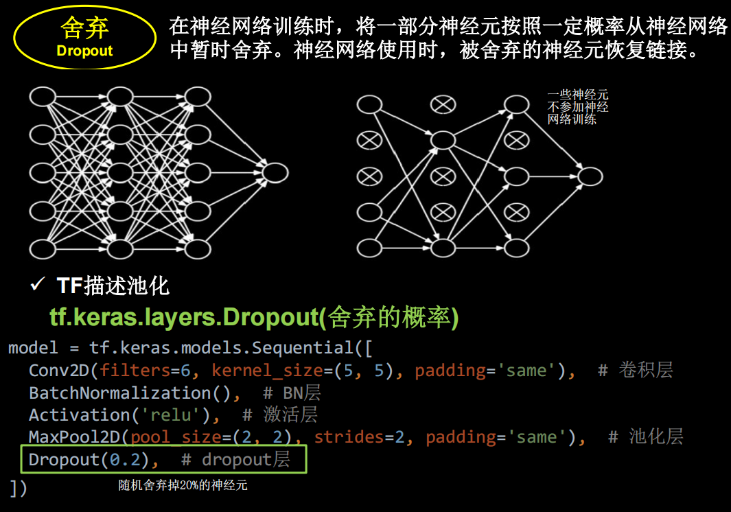
在神经网络的训练过程中,对于一次迭代中的某一层神经网络,先随机选择其中的一些神经元并将其临时丢弃,然后再进行本次的训练和优化。在下一次迭代中,继续随机隐藏一些神经元,直至训练结束。由于是随机丢弃,故而每一个批次都在训练不同的网络。
- 然后把输入x 通过修改后的网络前向传播,然后把得到的损失结果通过修改的网络反向传播。一小批(这里的批次batch_size由自己设定)训练样本执行完这个过程后,在没有被删除的神经元上按照随机梯度下降法更新对应的参数(w,b)
- 重复以下过程:
1、恢复被删掉的神经元(此时被删除的神经元保持原样,而没有被删除的神经元已经有所更新),因此每一个mini- batch都在训练不同的网络。
2、从隐藏层神经元中随机选择一个一半大小的子集临时删除掉(备份被删除神经元的参数)。
3、对一小批训练样本,先前向传播然后反向传播损失并根据随机梯度下降法更新参数(w,b) (没有被删除的那一部分参数得到更新,删除的神经元参数保持被删除前的结果)。
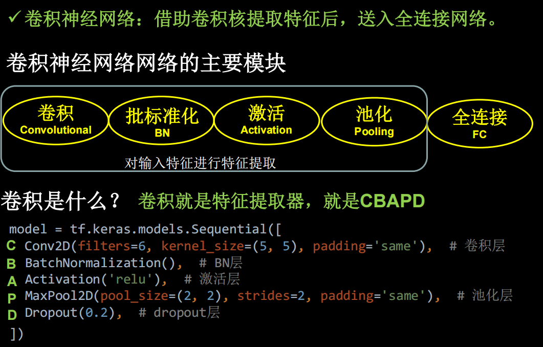
卷积神经网络
Cifar10数据集
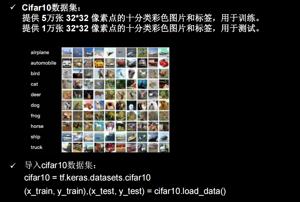
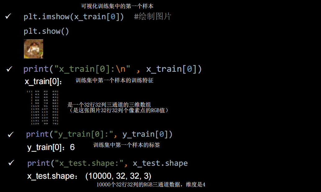
可视化部分样本
import tensorflow as tf
import numpy as np
import matplotlib.pyplot as plt
np.set_printoptions(threshold=np.inf)

data_cifar10=tf.keras.datasets.cifar10.load_data()
(x_train, y_train), (x_test, y_test) =data_cifar10

print(x_train.shape)
print(y_train.shape)
plt.imshow(x_train[0])
plt.show()
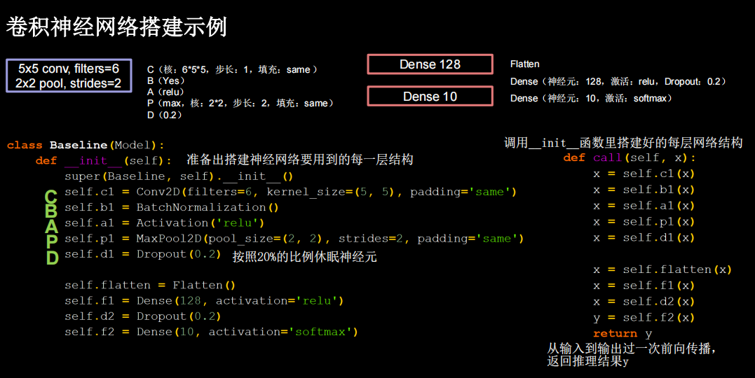
卷积神经网络搭建示例
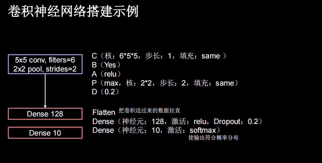
一层卷积两层全连接
import matplotlib.pyplot as plt
import tensorflow as tf
from tensorflow.keras.layers import Dense, Dropout,MaxPooling2D,Flatten,Conv2D,BatchNormalization
from tensorflow.keras import Model
import os
import numpy as np
from tensorflow_core.python.keras.layers import Activation
# np.set_printoptions(threshold=np.inf)


class Baseline(Model):
    def __init__(self):
        super(Baseline, self).__init__()
        self.conv1 = Conv2D(6, (5,5), padding='same')
        self.bn1 = BatchNormalization()
        self.a1= Activation('relu')
        self.pool1 = MaxPooling2D(pool_size=(2,2),strides=2,padding='same')
        self.d1=Dropout(0.2)

        self.flatten1 = Flatten()
        self.f1=Dense(128,activation='relu')
        self.d2=Dropout(0.2)
        self.f2=Dense(10,activation='softmax')

    def call(self,x):
        x = self.conv1(x)
        x = self.bn1(x)
        x = self.a1(x)
        x = self.pool1(x)
        x = self.d1(x)

        x = self.flatten1(x)
        x = self.f1(x)
        x =self.d2(x)
        y= self.f2(x)
        return y


(x_train, y_train), (x_test, y_test) = tf.keras.datasets.cifar10.load_data()
x_train,x_test = x_train/255.0,x_test/255.0


model = Baseline()
model.compile(optimizer=tf.keras.optimizers.Adam(lr=0.001),loss=tf.keras.losses.SparseCategoricalCrossentropy(from_logits=False)
              ,metrics=['sparse_categorical_accuracy'])

checkpoint_save_path="baseline.ckpt"
if os.path.exists(checkpoint_save_path+'.index'):
    model.load_weights(checkpoint_save_path)
    print("---------------------Loaded model---------------")

cp_callback = tf.keras.callbacks.ModelCheckpoint(filepath=checkpoint_save_path, save_weights_only=True
                                              ,save_best_only=True, verbose=1)


history=model.fit(x_train,y_train,batch_size=32, epochs=5, validation_data=(x_test, y_test)
          ,validation_freq=1,callbacks=[cp_callback])
model.summary()

file=open('weights.txt','w')
for v in model.trainable_variables:
    file.write(str(v.name)+'\n')
    file.write(str(v.shape)+'\n')
    file.write(str(v.numpy())+'\n')
file.close()

train_acc=history.history['sparse_categorical_accuracy']
val_acc=history.history['val_sparse_categorical_accuracy']
loss=history.history['loss']
val_loss=history.history['val_loss']

plt.subplot(1,2,1)
plt.plot(loss,label='train_loss')
plt.plot(val_loss,label='val_loss')
plt.title('model loss')
plt.legend()

plt.subplot(1,2,2)
plt.plot(train_acc,label='train_acc')
plt.plot(val_acc,label='val_acc')
plt.title('model acc')
plt.legend()
plt.show()
如果你是看到曹老师的课,这里你会遇到一个问题,准确率一直在0.1,因为30和40系显卡不支持老版本了,解决方法看这篇文章
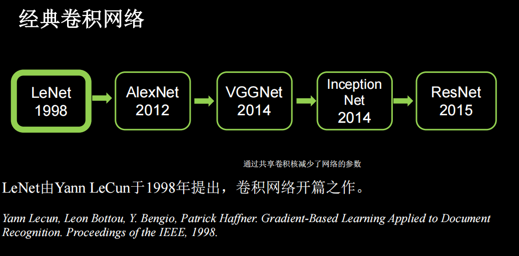
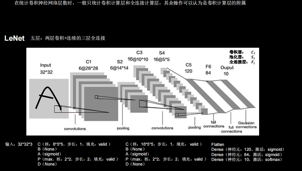
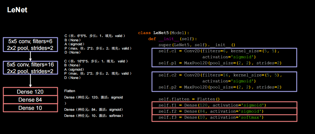
LeNet
import matplotlib.pyplot as plt
import tensorflow as tf
from tensorflow.keras.layers import Dense, Dropout,MaxPooling2D,Flatten,Conv2D,BatchNormalization,Activation
from tensorflow.keras import Model
import os
import numpy as np

# np.set_printoptions(threshold=np.inf)


class Baseline(Model):
    def __init__(self):
        super(Baseline, self).__init__()
        self.conv1 = Conv2D(6, (5,5), activation='sigmoid')
        self.pool1 = MaxPooling2D(pool_size=(2,2),strides=2)
        self.conv2 = Conv2D(16, (5,5), activation='sigmoid')
        self.pool2 = MaxPooling2D(pool_size=(2,2),strides=2)

        self.flatten1 = Flatten()
        self.f1=Dense(120,activation='sigmoid')
        self.f2=Dense(84,activation='sigmoid')
        self.f3=Dense(10,activation='softmax')

    def call(self,x):
        x = self.conv1(x)
        x = self.pool1(x)
        x = self.conv2(x)
        x = self.pool2(x)

        x = self.flatten1(x)
        x = self.f1(x)
        x = self.f2(x)
        y = self.f3(x)
        return y


(x_train, y_train), (x_test, y_test) = tf.keras.datasets.cifar10.load_data()
x_train,x_test = x_train/255.0,x_test/255.0


model = Baseline()
model.compile(optimizer=tf.keras.optimizers.Adam(lr=0.001),loss=tf.keras.losses.SparseCategoricalCrossentropy(from_logits=False)
              ,metrics=['sparse_categorical_accuracy'])

checkpoint_save_path="./checkpoints/lenet.ckpt"
if os.path.exists(checkpoint_save_path+'.index'):
    model.load_weights(checkpoint_save_path)
    print("---------------------Loaded model---------------")

cp_callback = tf.keras.callbacks.ModelCheckpoint(filepath=checkpoint_save_path, save_weights_only=True
                                              ,save_best_only=True, verbose=1)


history=model.fit(x_train,y_train,batch_size=32, epochs=5, validation_data=(x_test, y_test)
          ,validation_freq=1,callbacks=[cp_callback])
model.summary()

file=open('./checkpoints/weights_lenet.txt','w')
for v in model.trainable_variables:
    file.write(str(v.name)+'\n')
    file.write(str(v.shape)+'\n')
    file.write(str(v.numpy())+'\n')
file.close()

train_acc=history.history['sparse_categorical_accuracy']
val_acc=history.history['val_sparse_categorical_accuracy']
loss=history.history['loss']
val_loss=history.history['val_loss']

plt.subplot(1,2,1)
plt.plot(loss,label='train_loss')
plt.plot(val_loss,label='val_loss')
plt.title('model loss')
plt.legend()

plt.subplot(1,2,2)
plt.plot(train_acc,label='train_acc')
plt.plot(val_acc,label='val_acc')
plt.title('model acc')
plt.legend()
plt.show()
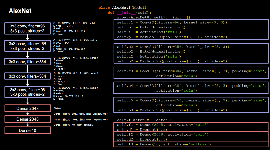
AlexNet

共8层
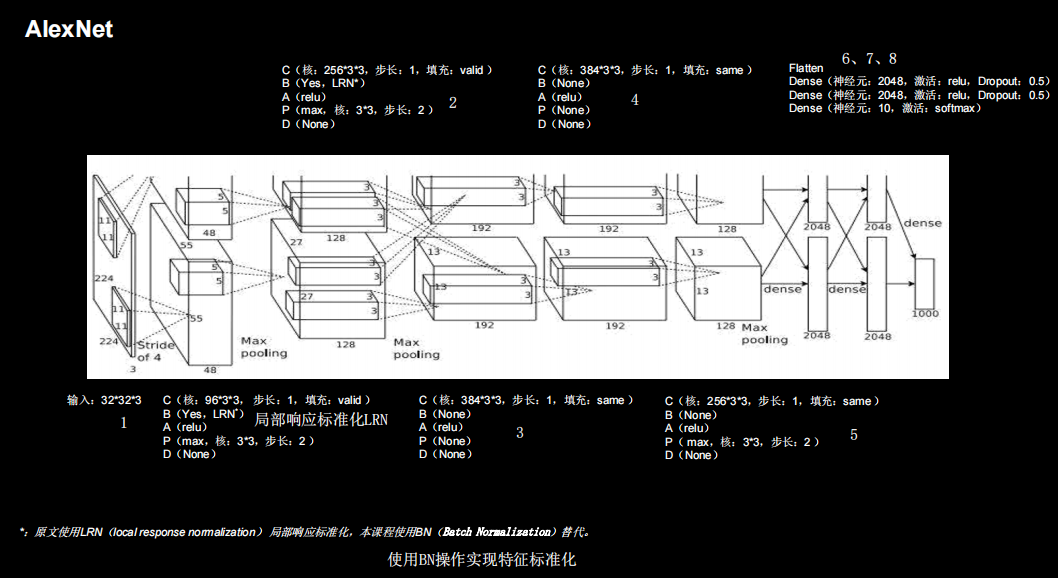
网络架构
import matplotlib.pyplot as plt
import tensorflow as tf
from tensorflow.keras.layers import Dense, Dropout,MaxPooling2D,Flatten,Conv2D,BatchNormalization,Activation,Flatten
from tensorflow.keras import Model
import os
import numpy as np

# np.set_printoptions(threshold=np.inf)


class AlexNet(Model):
    def __init__(self):
        super(AlexNet, self).__init__()
        self.conv1 = Conv2D(96, kernel_size=(3,3), padding='valid')
        self.bn1 = BatchNormalization()
        self.a1= Activation('relu')
        self.pool1 = MaxPooling2D(pool_size=(3,3),strides=2)

        self.conv2 = Conv2D(256, (3,3), padding='valid')
        self.bn2 = BatchNormalization()
        self.a2= Activation('relu')
        self.pool2 = MaxPooling2D(pool_size=(3,3),strides=2)

        self.conv3 = Conv2D(384, (3,3), padding='same',activation='relu')

        self.conv4 = Conv2D(384, (3,3), padding='same',activation='relu')

        self.conv5 = Conv2D(256, (3,3), padding='same',activation='relu')
        self.pool5 = MaxPooling2D(pool_size=(3,3),strides=2)

        self.flatten1 = Flatten()
        self.f1=Dense(2048,activation='relu')
        self.d1=Dropout(0.5)
        self.f2=Dense(2048,activation='relu')
        self.d2=Dropout(0.5)
        self.f3=Dense(10,activation='softmax')

    def call(self,x):
        x=self.conv1(x)
        x=self.bn1(x)
        x=self.a1(x)
        x=self.pool1(x)

        x=self.conv2(x)
        x=self.bn2(x)
        x=self.a2(x)
        x=self.pool2(x)

        x=self.conv3(x)

        x=self.conv4(x)

        x=self.conv5(x)
        x=self.pool5(x)

        x=self.flatten1(x)
        x=self.f1(x)
        x=self.d1(x)
        x=self.f2(x)
        x=self.d2(x)
        y=self.f3(x)
        return y


(x_train, y_train), (x_test, y_test) = tf.keras.datasets.cifar10.load_data()
x_train,x_test = x_train/255.0,x_test/255.0


model = AlexNet()
model.compile(optimizer='Adam',loss=tf.keras.losses.SparseCategoricalCrossentropy(from_logits=False)
              ,metrics=['sparse_categorical_accuracy'])

checkpoint_save_path="./checkpoints/Alex.ckpt"
if os.path.exists(checkpoint_save_path+'.index'):
    model.load_weights(checkpoint_save_path)
    print("---------------------Loaded model---------------")

cp_callback = tf.keras.callbacks.ModelCheckpoint(filepath=checkpoint_save_path, save_weights_only=True
                                              ,save_best_only=True, verbose=1)


history=model.fit(x_train,y_train,batch_size=32, epochs=5, validation_data=(x_test, y_test)
          ,validation_freq=1,callbacks=[cp_callback])
model.summary()

file=open('./checkpoints/weights_alex.txt','w')
for v in model.trainable_variables:
    file.write(str(v.name)+'\n')
    file.write(str(v.shape)+'\n')
    file.write(str(v.numpy())+'\n')
file.close()

train_acc=history.history['sparse_categorical_accuracy']
val_acc=history.history['val_sparse_categorical_accuracy']
loss=history.history['loss']
val_loss=history.history['val_loss']

plt.subplot(1,2,1)
plt.plot(loss,label='train_loss')
plt.plot(val_loss,label='val_loss')
plt.title('model loss')
plt.legend()

plt.subplot(1,2,2)
plt.plot(train_acc,label='train_acc')
plt.plot(val_acc,label='val_acc')
plt.title('model acc')
plt.legend()
plt.show()
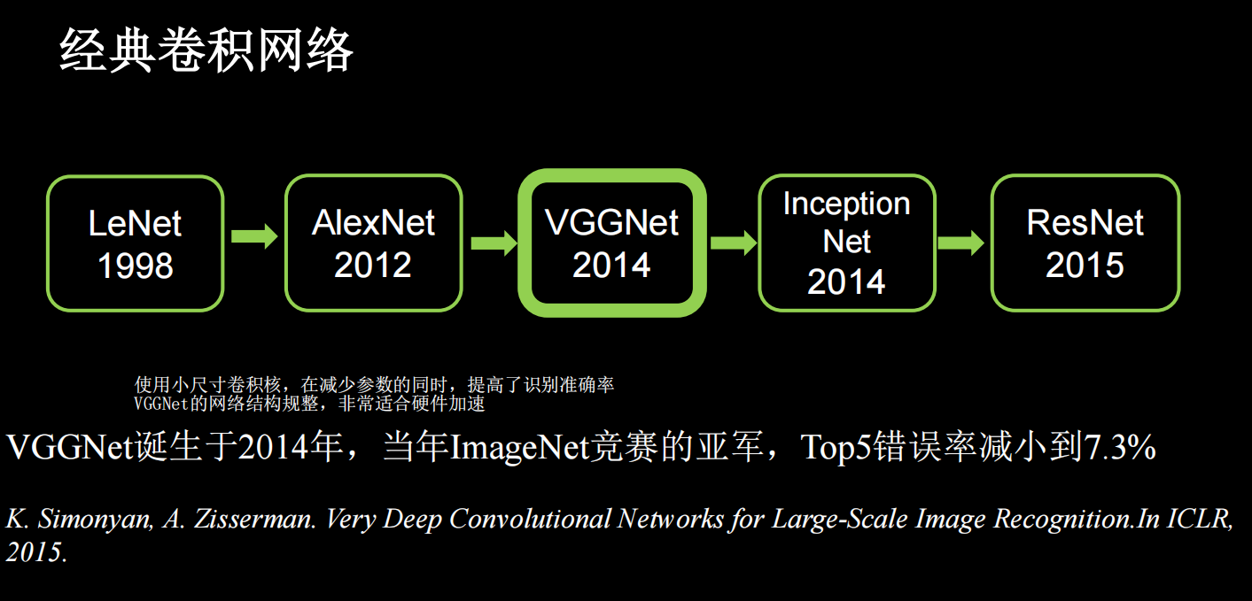
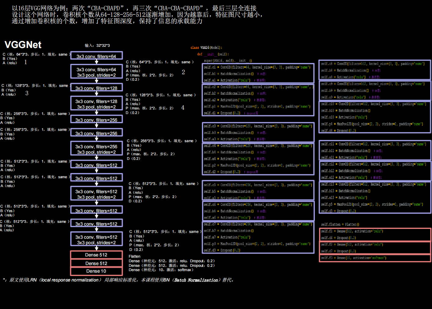
VGGNet
import matplotlib.pyplot as plt
import tensorflow as tf
from tensorflow.keras.layers import Dense, Dropout,MaxPooling2D,Flatten,Conv2D,BatchNormalization,Activation,Flatten
from tensorflow.keras import Model
import os
import numpy as np

# np.set_printoptions(threshold=np.inf)


class VGG16(Model):
    def __init__(self):
        super(VGG16, self).__init__()
        self.conv1 = Conv2D(64, (3, 3),padding='same')
        self.bn1 = BatchNormalization()
        self.a1= Activation('relu')

        self.conv2 = Conv2D(64, (3, 3),padding='same')
        self.bn2 = BatchNormalization()
        self.a2= Activation('relu')
        self.pool2 = MaxPooling2D((2, 2), strides=2,padding='same')
        self.d2=Dropout(0.2)

        self.conv3 = Conv2D(128, (3, 3),padding='same')
        self.bn3= BatchNormalization()
        self.a3= Activation('relu')

        self.conv4 = Conv2D(128, (3, 3),padding='same')
        self.bn4=BatchNormalization()
        self.a4= Activation('relu')
        self.p4= MaxPooling2D((2, 2), strides=2,padding='same')
        self.d4= Dropout(0.2)

        self.conv5 = Conv2D(256, (3, 3),padding='same')
        self.bn5=BatchNormalization()
        self.a5= Activation('relu')

        self.conv6= Conv2D(256, (3, 3),padding='same')
        self.bn6= BatchNormalization()
        self.a6= Activation('relu')

        self.conv7= Conv2D(256, (3, 3),padding='same')
        self.bn7= BatchNormalization()
        self.a7= Activation('relu')
        self.p7= MaxPooling2D((2, 2), strides=2,padding='same')
        self.d7= Dropout(0.2)

        self.conv8= Conv2D(512, (3, 3),padding='same')
        self.bn8=BatchNormalization()
        self.a8= Activation('relu')

        self.conv9= Conv2D(512, (3, 3),padding='same')
        self.bn9= BatchNormalization()
        self.a9= Activation('relu')

        self.conv10= Conv2D(512, (3, 3),padding='same')
        self.bn10= BatchNormalization()
        self.a10= Activation('relu')
        self.p10= MaxPooling2D((2, 2), strides=2,padding='same')
        self.d10= Dropout(0.2)

        self.conv11= Conv2D(512, (3, 3),padding='same')
        self.bn11= BatchNormalization()
        self.a11= Activation('relu')

        self.conv12= Conv2D(512, (3, 3),padding='same')
        self.bn12= BatchNormalization()
        self.a12= Activation('relu')

        self.conv13= Conv2D(512, (3, 3),padding='same')
        self.bn13= BatchNormalization()
        self.a13= Activation('relu')
        self.p13= MaxPooling2D((2, 2), strides=2,padding='same')
        self.d13= Dropout(0.2)

        self.flatten= Flatten()
        self.fc14= Dense(512,activation='relu')
        self.d14=Dropout(0.2)
        self.fc15= Dense(512,activation='relu')
        self.d15= Dropout(0.2)
        self.fc16=Dense(10,activation='softmax')


    def call(self,x):
        x = self.conv1(x)
        x=self.bn1(x)
        x=self.a1(x)

        x=self.conv2(x)
        x=self.bn2(x)
        x=self.a2(x)
        x=self.pool2(x)
        x=self.d2(x)

        x=self.conv3(x)
        x=self.bn3(x)
        x=self.a3(x)

        x=self.conv4(x)
        x=self.bn4(x)
        x=self.a4(x)
        x=self.p4(x)
        x=self.d4(x)

        x=self.conv5(x)
        x=self.bn5(x)
        x=self.a5(x)

        x=self.conv6(x)
        x=self.bn6(x)
        x=self.a6(x)

        x=self.conv7(x)
        x=self.bn7(x)
        x=self.a7(x)
        x=self.p7(x)
        x=self.d7(x)

        x=self.conv8(x)
        x=self.bn8(x)
        x=self.a8(x)

        x=self.conv9(x)
        x=self.bn9(x)
        x=self.a9(x)

        x=self.conv10(x)
        x=self.bn10(x)
        x=self.a10(x)
        x=self.p10(x)
        x=self.d10(x)

        x=self.conv11(x)
        x=self.bn11(x)
        x=self.a11(x)

        x=self.conv12(x)
        x=self.bn12(x)
        x=self.a12(x)

        x=self.conv13(x)
        x=self.bn13(x)
        x=self.a13(x)
        x=self.p13(x)
        x=self.d13(x)

        x=self.flatten(x)
        x=self.fc14(x)
        x=self.fc15(x)
        y=self.fc16(x)
        return y


(x_train, y_train), (x_test, y_test) = tf.keras.datasets.cifar10.load_data()
x_train,x_test = x_train/255.0,x_test/255.0


model = VGG16()
model.compile(optimizer='Adam',loss=tf.keras.losses.SparseCategoricalCrossentropy(from_logits=False)
              ,metrics=['sparse_categorical_accuracy'])

checkpoint_save_path="./checkpoints/VGG16.ckpt"
if os.path.exists(checkpoint_save_path+'.index'):
    model.load_weights(checkpoint_save_path)
    print("---------------------Loaded model---------------")

cp_callback = tf.keras.callbacks.ModelCheckpoint(filepath=checkpoint_save_path, save_weights_only=True
                                              ,save_best_only=True, verbose=1)


history=model.fit(x_train,y_train,batch_size=32, epochs=5, validation_data=(x_test, y_test)
          ,validation_freq=1,callbacks=[cp_callback])
model.summary()

file=open('./checkpoints/weights_VGG16.txt','w')
for v in model.trainable_variables:
    file.write(str(v.name)+'\n')
    file.write(str(v.shape)+'\n')
    file.write(str(v.numpy())+'\n')
file.close()

train_acc=history.history['sparse_categorical_accuracy']
val_acc=history.history['val_sparse_categorical_accuracy']
loss=history.history['loss']
val_loss=history.history['val_loss']

plt.subplot(1,2,1)
plt.plot(loss,label='train_loss')
plt.plot(val_loss,label='val_loss')
plt.title('model loss')
plt.legend()

plt.subplot(1,2,2)
plt.plot(train_acc,label='train_acc')
plt.plot(val_acc,label='val_acc')
plt.title('model acc')
plt.legend()
plt.show()
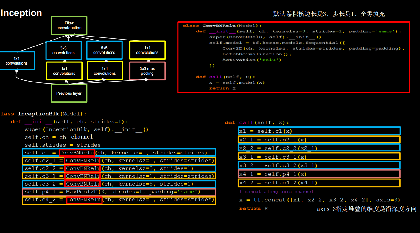
Inception

引入Inception结构块,在同一层网络内使用不同尺寸的卷积核,提升了模型感知力;使用了批标准化,缓解了梯度消失。
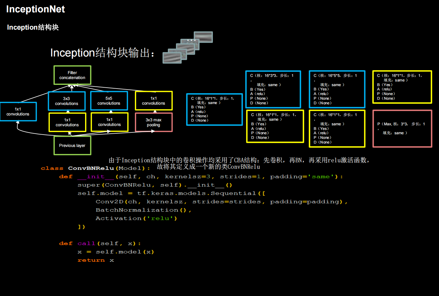
核心是它的基本单元Inception结构块,无论是GoogLeNet(Inception v1),还是InceptionNet的后续版本,比如v2/v3/v4,
都是基于Inception结构块搭建的网络。Inception结构块在同一层网络中使用了多个尺寸的卷积核,可以提取不同尺寸的特征。
通过1×1卷积核作用到输入特征图的每个像素点,通过设定少于输入特征图深度的1*1卷积核个数,减少了输出特征图深度,起到
了降维的作用,减少了参数量和计算量。
Inception有四个分支,具体结构见上图右上角
里面有很多重复的代码,编写ConvBNRelu类,增加代码可读性。
有了Inception块后,就能搭建精简版本的InceptionNet
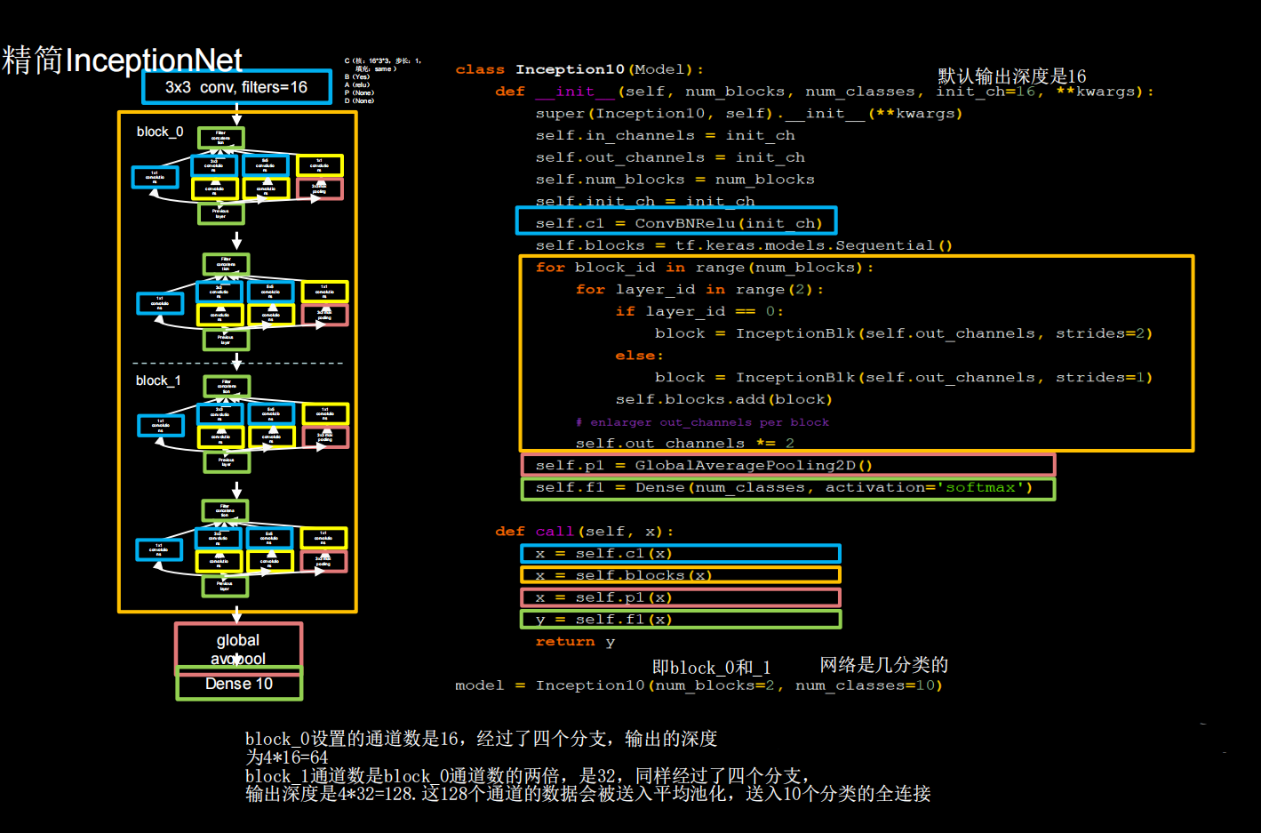
网络共有10层,第一次是一个3×3的conv,然后是4个Inception结构块顺序相连,每两个Inception结构块组成一个block每个block中的第一个Inception结构块卷积步长是2,第二个Inception结构块卷积步长是1,这使得第一个Inception结构块输出特征图尺寸减半,因此把输出特征图深度加深,尽可能保证特征抽取中信息的承载量一致。
block_0设置的卷积核个数是16,经过了四个分支,输出的深度为4 * 16=64。block_1卷积核个数是block_0通的两倍(self.out_channels * = 2),是32,同样经过了四个分支,输出深度是4*32=128.这128个通道的数据会被送入平均池化,送入10个分类的全连接

首先我们简单理解全局平均池化操作。之前我们需要把特征图展开然后进行全连接,而现在,我们直接没有了这一步。
如果有一批特征图,其尺寸为 [ B, C, H, W], 我们经过全局平均池化之后,尺寸变为[B, C, 1, 1]。
也就是说,全局平均池化其实就是对每一个通道图所有像素值求平均值,然后得到一个新的1 * 1的通道图。
由于网络规模比较大,把batch_size调整到1024,让训练时一次喂入神经网络的数据量多一些,以充分发挥显卡的性能,提高训练速度
一般让显卡达到70-80%的负荷比较合理。注意:数据量大的时候可以调大batchsize,数据量小的时候batchsize不要调太大,因为数据量小的时候,如果batchsize小,那么一个epoch会有很多batchsize,每一个batchsize都会进行梯度更新。
import matplotlib.pyplot as plt
import tensorflow as tf
from tensorflow.keras.layers import Dense, Dropout,MaxPooling2D,Flatten,Conv2D,BatchNormalization,\
    Activation,Flatten,GlobalAveragePooling2D
from tensorflow.keras import Model, Sequential
import os
import numpy as np

# np.set_printoptions(threshold=np.inf)


class ConvBNRelu(Model):
    def __init__(self,filters,kernel_size,stride=1):
        super(ConvBNRelu, self).__init__()
        self.model = Sequential([
            Conv2D(filters, kernel_size,strides=stride, padding='same'),
            BatchNormalization(),
            Activation('relu'),
        ])

    def call(self,x):
        y=self.model(x,training=False)
        return y


class Inception(Model):
    def __init__(self,init_ch,stride):
        super(Inception, self).__init__()
        self.c1=ConvBNRelu(init_ch,1,stride=stride)  # 方便下面Inception10控制特征图的size
        self.c2_1=ConvBNRelu(init_ch,1,stride=stride) #
        self.c2_2=ConvBNRelu(init_ch,3)
        self.c3_1=ConvBNRelu(init_ch,1,stride=stride) #
        self.c3_2=ConvBNRelu(init_ch,5)
        self.c4_1=MaxPooling2D((3,3),strides=(1,1),padding='same')
        self.c4_2=ConvBNRelu(init_ch,1,stride=stride)  #

    def call(self,x):
        x1=self.c1(x)  # x=self.c1(x)
        x2=self.c2_1(x)
        x2=self.c2_2(x2)
        x3=self.c3_1(x)
        x3=self.c3_2(x3)
        x4=self.c4_1(x)
        x4=self.c4_2(x4)
        y=tf.concat([x1,x2,x3,x4],axis=3)
        return y


class Inception10(Model):
    def __init__(self,num_classes,block_n,init_ch=16):
        super(Inception10,self).__init__()
        self.channel=init_ch   # 卷积核个数
        self.blocks=Sequential()
        self.c1=ConvBNRelu(16,3)  # 最开头的那一层
        for i in range(block_n):
            for j in range(2):
                if j%2==0:
                    block=Inception(self.channel,stride=2)
                else:
                    block=Inception(self.channel,stride=1)
                self.blocks.add(block)   #
            self.channel*=2     # stride=2会使特征图size变小,通过增加channnel来表示更多信息
        self.pool=GlobalAveragePooling2D()
        self.dense=Dense(num_classes,activation='softmax')

    def call(self,x):
        x=self.c1(x)
        x = self.blocks(x)
        x = self.pool(x)
        x = self.dense(x)
        return x

(x_train, y_train), (x_test, y_test) = tf.keras.datasets.cifar10.load_data()
x_train,x_test = x_train/255.0,x_test/255.0


model = Inception10(10,block_n=2)
model.compile(optimizer='Adam',loss=tf.keras.losses.SparseCategoricalCrossentropy(from_logits=False)
              ,metrics=['sparse_categorical_accuracy'])

checkpoint_save_path="./checkpoints/Inception10_gai2.ckpt"
if os.path.exists(checkpoint_save_path+'.index'):
    model.load_weights(checkpoint_save_path)
    print("---------------------Loaded model---------------")

cp_callback = tf.keras.callbacks.ModelCheckpoint(filepath=checkpoint_save_path, save_weights_only=True
                                              ,save_best_only=True, verbose=1)


history=model.fit(x_train,y_train,batch_size=32, epochs=5, validation_data=(x_test, y_test)
          ,validation_freq=1,callbacks=[cp_callback])
model.summary()

file=open('./checkpoints/weights_Inception10_gai2.txt','w')
for v in model.trainable_variables:
    file.write(str(v.name)+'\n')
    file.write(str(v.shape)+'\n')
    file.write(str(v.numpy())+'\n')
file.close()

train_acc=history.history['sparse_categorical_accuracy']
val_acc=history.history['val_sparse_categorical_accuracy']
loss=history.history['loss']
val_loss=history.history['val_loss']

plt.subplot(1,2,1)
plt.plot(loss,label='train_loss')
plt.plot(val_loss,label='val_loss')
plt.title('model loss')
plt.legend()

plt.subplot(1,2,2)
plt.plot(train_acc,label='train_acc')
plt.plot(val_acc,label='val_acc')
plt.title('model acc')
plt.legend()
plt.show()
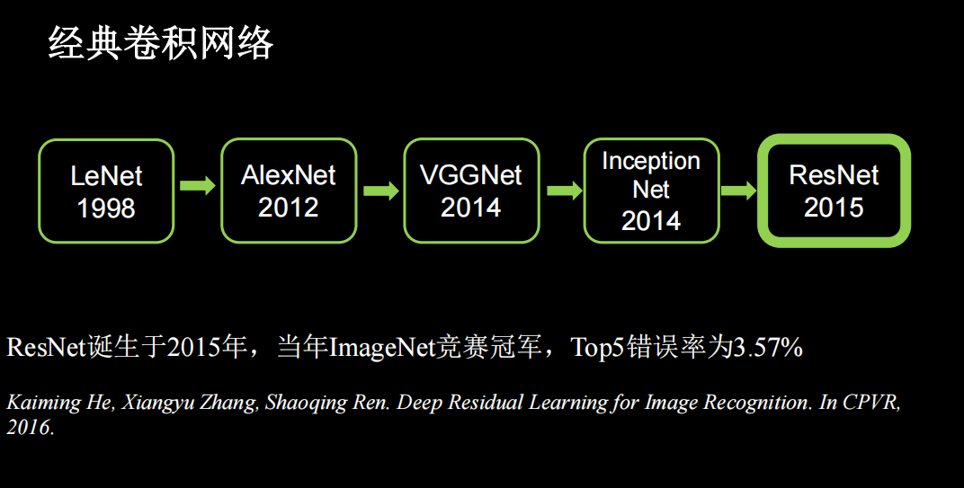
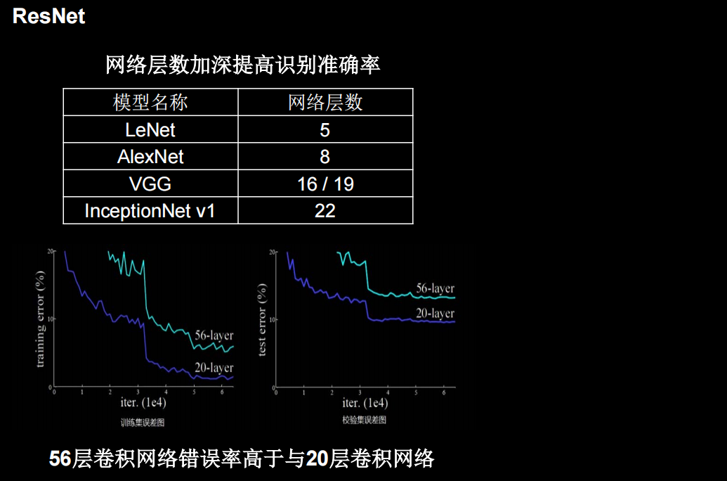
ResNet
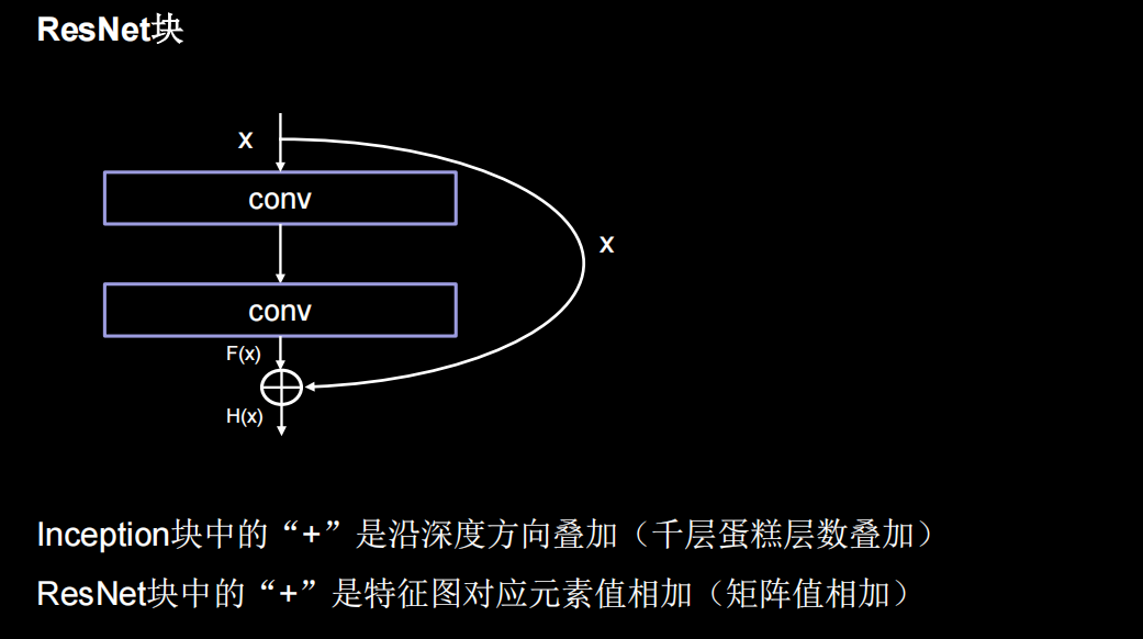
提出了层间残差跳连,引入了前方信息,缓解梯度消失,使神经网络层数增加成为可能
单纯堆叠神经网络层数会使神经网络模型退化,以至于后边的特征丢失了前边特征的原本模样
用了一根跳连线,将前边的特征直接接到了后边,使输出结果H(x)包含了堆叠卷积的非线性输出F(x),和跳过这两层堆叠卷积、直接连接过来的恒等映射x,让它们对应元素相加。这一操作有效缓解了神经网络模型堆叠导致的退化,使得神经网络可以向着更深层级发展。
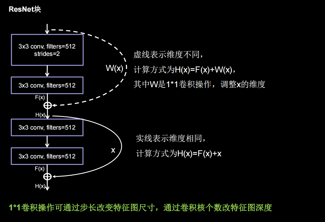
ResNet块中有两种情况,一种是用下图实线表示,两层堆叠卷积没有改变特征图的维度,即特征图的个数、高、宽和深度都相同,可以直接将F(x)与x相加。另一种情况用虚线表示,两层堆叠卷积改变了特征图的维度,需要借助1*1的卷积来调整x的维度,使W(x)与F(x)维度一致
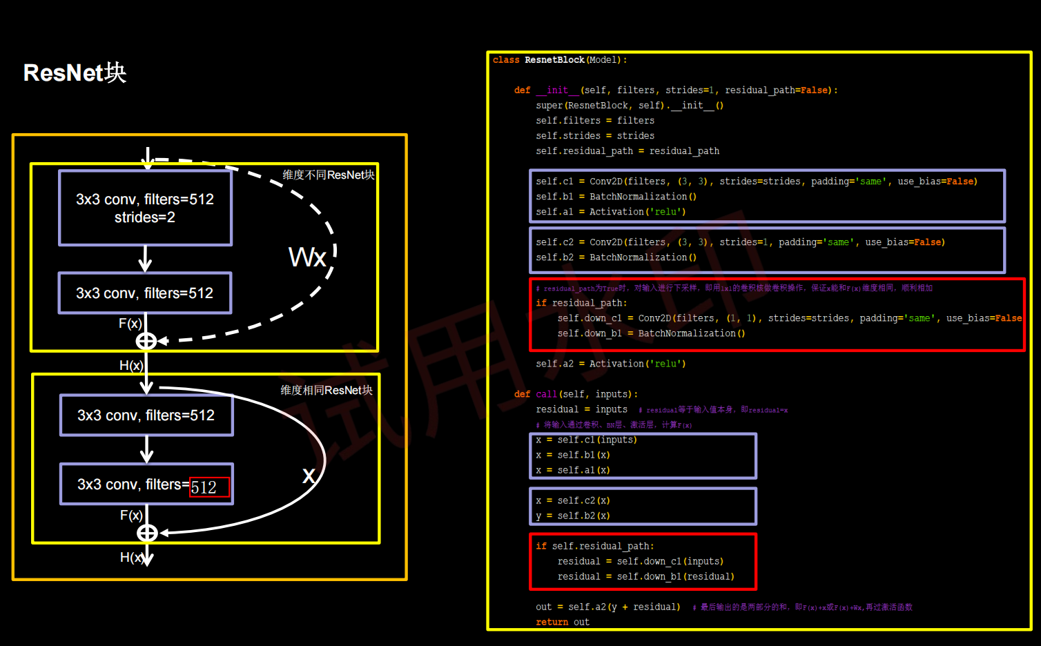
如果堆叠卷积层前后维度不同,residual_path=1,使用1*1卷积操作调整输入特征图inputs的尺寸或深度后,将堆叠卷积输出特征y和if语句计算出的residual相加,过激活,输出如果堆叠卷积层前后维度相同,直接将堆叠卷积输出特征y和输入特征图inputs相加,过激活,输出。下面的黄色框就是一个block,橘黄色框里有两种不同情况的block
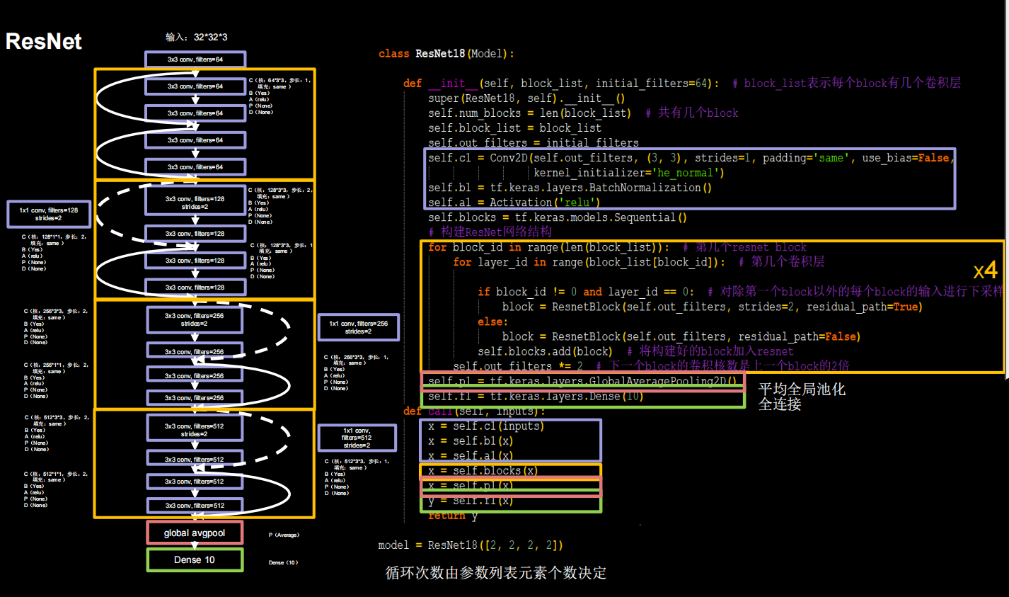
ResNet18:8个ResNet块,每一个ResNet块有两层卷积,一共是18层网络。为了加速模型收敛,把batch_size调到128
import matplotlib.pyplot as plt
import tensorflow as tf
from tensorflow.keras.layers import Dense, Dropout,MaxPooling2D,Flatten,Conv2D,BatchNormalization,\
    Activation,Flatten,GlobalAveragePooling2D
from tensorflow.keras import Model, Sequential
import os
import numpy as np

# np.set_printoptions(threshold=np.inf)


class ResNetBlock(Model):
    def __init__(self, filters, stride,residual):
        super(ResNetBlock, self).__init__()
        self.filters = filters
        self.strides = stride
        self.residual = residual

        self.conv1 = Conv2D(self.filters, 3, strides=self.strides,padding='same',use_bias=False)
        self.bn1 = BatchNormalization()
        self.a1= Activation('relu')

        self.conv2 = Conv2D(self.filters, 3, strides=1,padding='same',use_bias=False)
        self.bn2 = BatchNormalization()

        if residual:
            self.conv3 = Conv2D(self.filters, 1, strides=self.strides,padding='same',use_bias=False)
            self.bn3 = BatchNormalization()
        self.a2 = Activation('relu')

    def call(self, inputs,*args, **kwargs):
        resi = inputs
        x = self.conv1(inputs)
        x = self.bn1(x)
        x = self.a1(x)

        x = self.conv2(x)
        x = self.bn2(x)

        if self.residual:
            y=self.conv3(inputs)    #
            y=self.bn3(y)
            resi=y

        return self.a2(x+resi)


class ResNet18(Model):
    def __init__(self,block_list,init_channels,num_classes):
        super(ResNet18, self).__init__()
        self.conv1 = Conv2D(64,3,strides=1,padding='same',use_bias=False)
        self.bn1 = BatchNormalization()
        self.a1 = Activation('relu')

        self.ll=len(block_list)
        self.blocks=Sequential()
        for block_i in range(self.ll):
            for layer in range(block_list[block_i]):
                if block_i !=0 and layer==0:
                    self.blocks.add(ResNetBlock(init_channels,2,residual=True))
                else:
                    self.blocks.add(ResNetBlock(init_channels,1,residual=False))
            init_channels=init_channels*2
        self.p1=GlobalAveragePooling2D()
        self.f1=Dense(num_classes,activation='softmax',kernel_regularizer=tf.keras.regularizers.l2())

    def call(self, inputs,*args, **kwargs):
        x = self.conv1(inputs)
        x=self.bn1(x)
        x = self.a1(x)
        x=self.blocks(x)
        x=self.p1(x)
        x=self.f1(x)
        return x


(x_train, y_train), (x_test, y_test) = tf.keras.datasets.cifar10.load_data()
x_train,x_test = x_train/255.0,x_test/255.0


model = ResNet18([2,2,2,2],64,num_classes=10)
model.compile(optimizer='Adam',loss=tf.keras.losses.SparseCategoricalCrossentropy(from_logits=False)
              ,metrics=['sparse_categorical_accuracy'])

checkpoint_save_path="./checkpoints/ResNet18.ckpt"
if os.path.exists(checkpoint_save_path+'.index'):
    model.load_weights(checkpoint_save_path)
    print("---------------------Loaded model---------------")

cp_callback = tf.keras.callbacks.ModelCheckpoint(filepath=checkpoint_save_path, save_weights_only=True
                                              ,save_best_only=True, verbose=1)


history=model.fit(x_train,y_train,batch_size=32, epochs=5, validation_data=(x_test, y_test)
          ,validation_freq=1,callbacks=[cp_callback])
model.summary()

file=open('./checkpoints/weights_ResNet18txt','w')
for v in model.trainable_variables:
    file.write(str(v.name)+'\n')
    file.write(str(v.shape)+'\n')
    file.write(str(v.numpy())+'\n')
file.close()

train_acc=history.history['sparse_categorical_accuracy']
val_acc=history.history['val_sparse_categorical_accuracy']
loss=history.history['loss']
val_loss=history.history['val_loss']

plt.subplot(1,2,1)
plt.plot(loss,label='train_loss')
plt.plot(val_loss,label='val_loss')
plt.title('model loss')
plt.legend()

plt.subplot(1,2,2)
plt.plot(train_acc,label='train_acc')
plt.plot(val_acc,label='val_acc')
plt.title('model acc')
plt.legend()
plt.show()
可以比较一下这几个模型在cifar10上的表现,epoch=5,batchsize=32
| Model | train_acc | val_acc |
|---|---|---|
| baseline | 0.5469 | 0.4969 |
| LeNet | 0.4435 | 0.4407 |
| AlexNet | 0.6545 | 0.5186 |
| VGGNet | 0.7525 | 0.7039 |
| Inception10 | 0.7927 | 0.7444 |
| ResNet18 | 0.8688 | 0.7946 |
经典卷积网络小结

class6
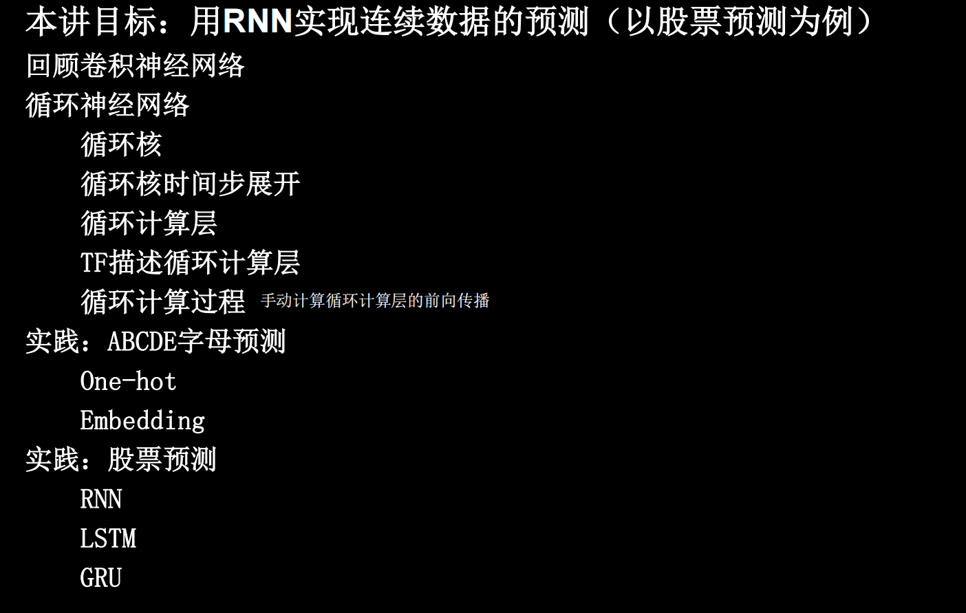
循环核
有些数据是和时间序列相关的,是可以根据上午预测出下文的

给你一段话,鱼离不开_,你可能下意识会说水,因为你记住了前面的四个,可以推出大概率是水
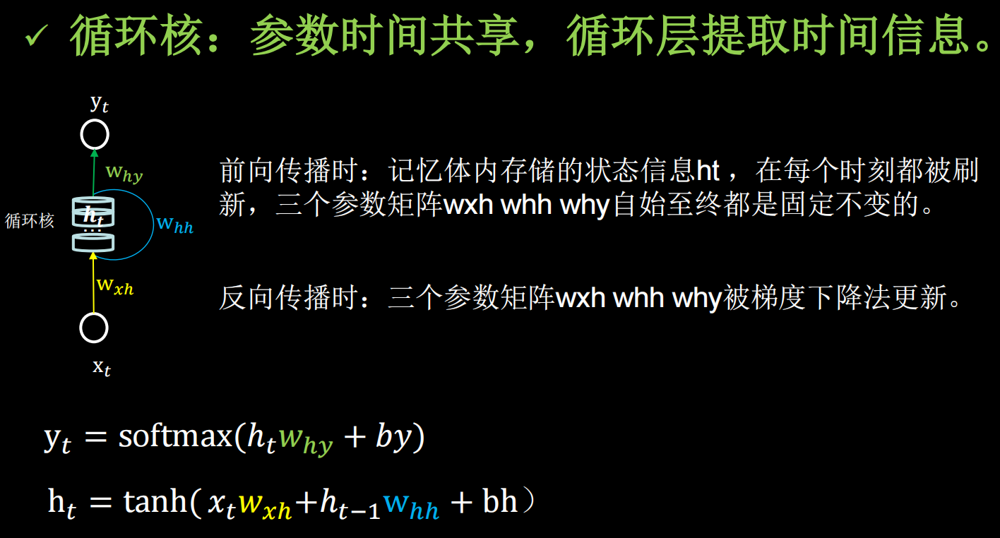
输入 x t x_t xt维度和输出 y t y_t yt的维度,以及循环核的个数确定,三个参数矩阵的维度也就确定了
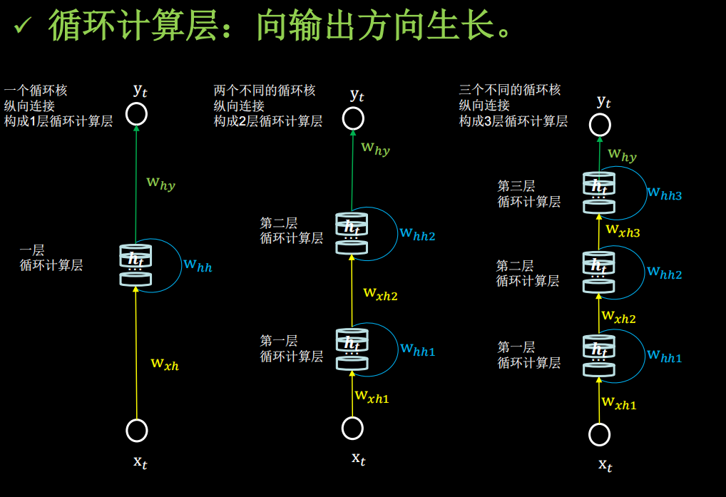
每一个循环核构成一个循环计算层
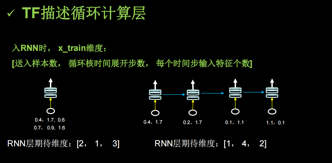
TF描述循环计算层
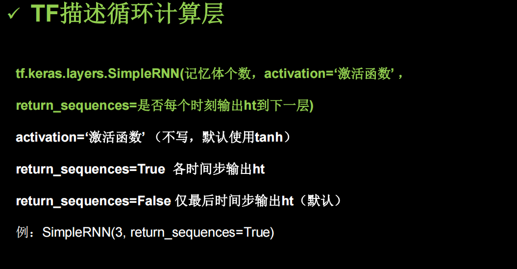
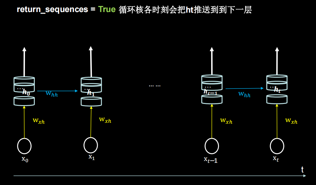
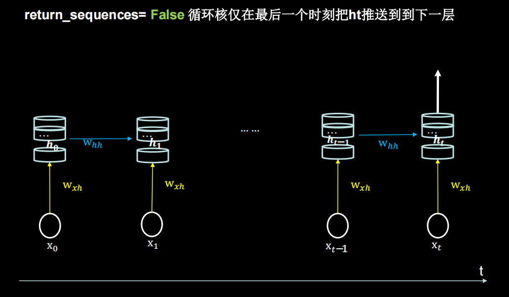
return_sequences设为False,True的区别如下(布尔。是返回输出序列中的最后一个输出,还是返回完整序列。默认值:False。)
对输入的样本维度有要求
循环计算过程 I
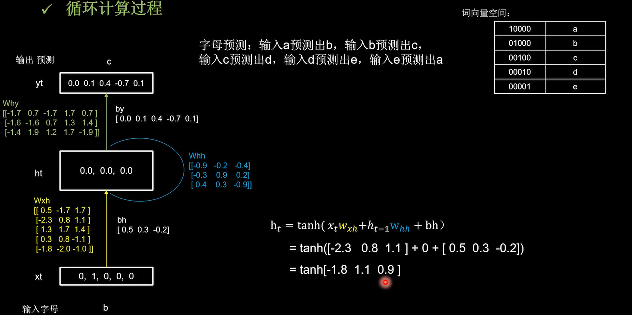
记忆体的个数为3, W h x , W h h , W h y W_{hx},W_{hh},W_{hy} Whx,Whh,Why是训练好的参数。过tanh激活函数后得到当前时刻的状态信息ht
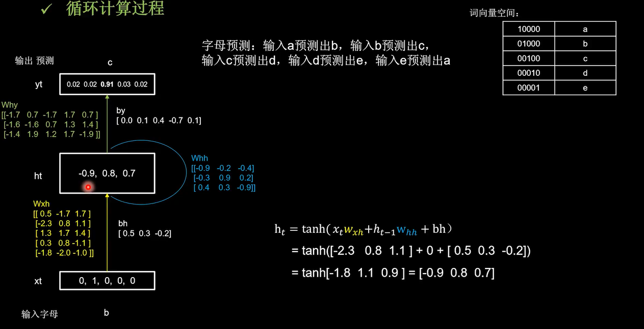
记忆体存储的状态信息被刷新为[-0.9,0.8,0.7],然后输出yt是把提取到的时间信息,通过全连接进行识别预测的过程,是整个网络的输出层
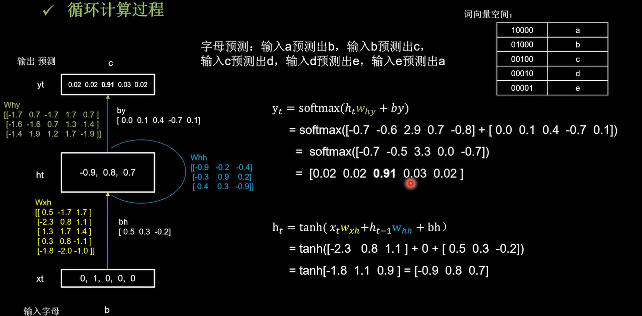
模型认为有91%的概率输出c。下面看一下代码实现
字母预测onehot_1pre1
用RNN实现输入一个字母,预测下一个字母(One hot 编码)
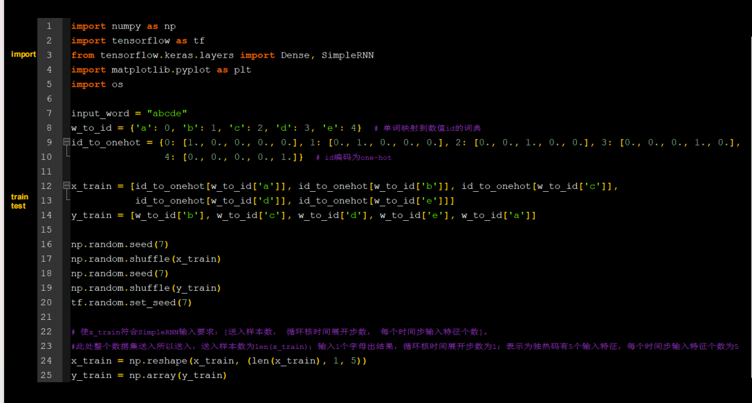
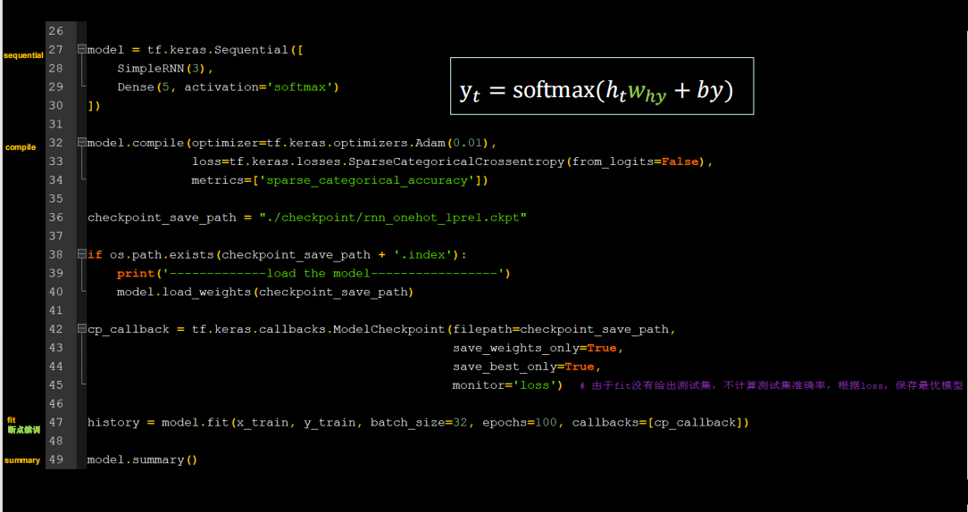
SimpleRNN(3),  # 这里可以自行调节记忆体个数
Dense(5, activation='softmax')  # 一层全连接,实现输出层yt的计算,由于要映射到独立热编码,找到最大概率字母,所以=5
代码
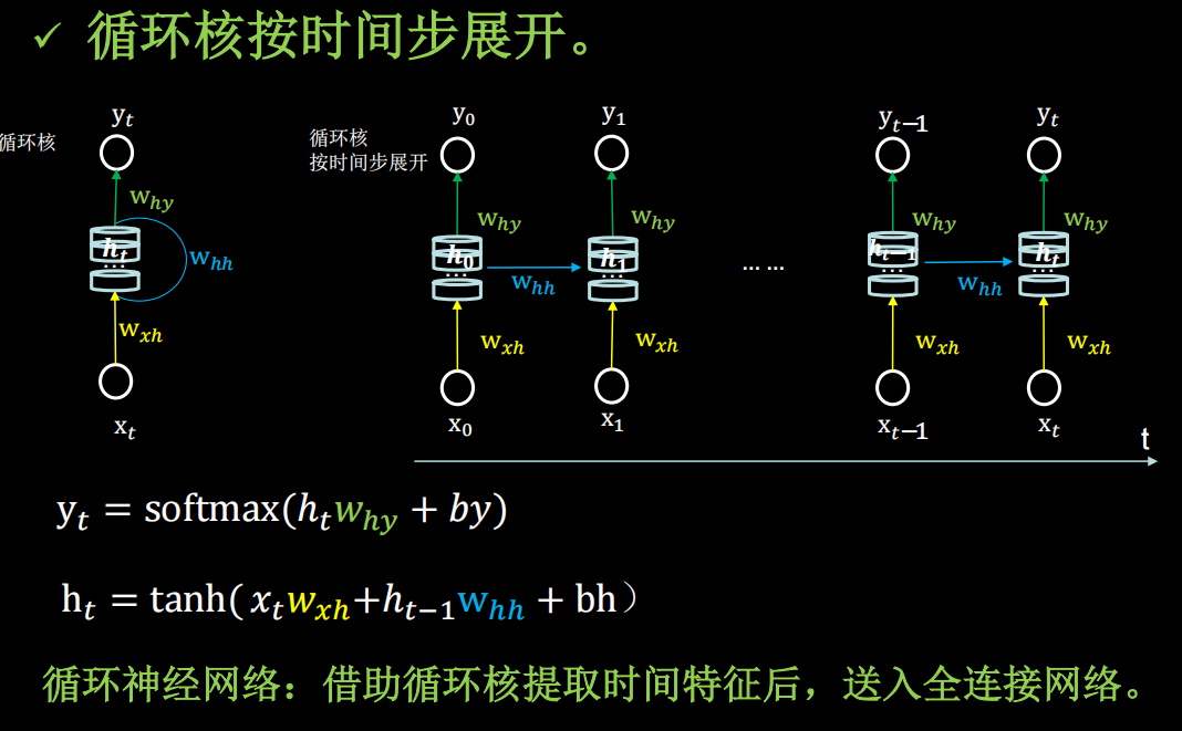
循环计算过程2
前面是输入是一个字母,预测下一个字母。现在感受一下把循环核按时间步展开,连续输入多个字母预测下一个字母。仍然使用三个记忆体,初始为0,用一套训练好的参数矩阵,带你感受循环计算的前向传播
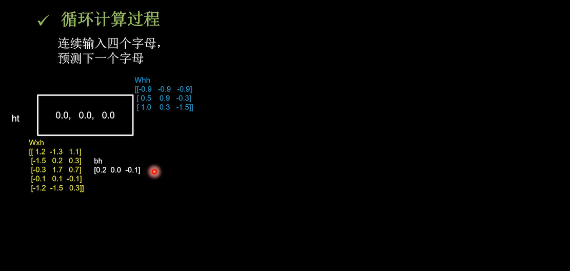
输入b更新记忆体
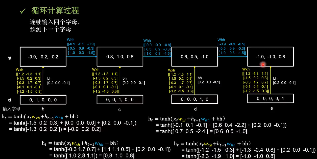
这四个时间步中所用到的参数矩阵,Wxh和bh是完全相同的。输出预测通过全连接完成
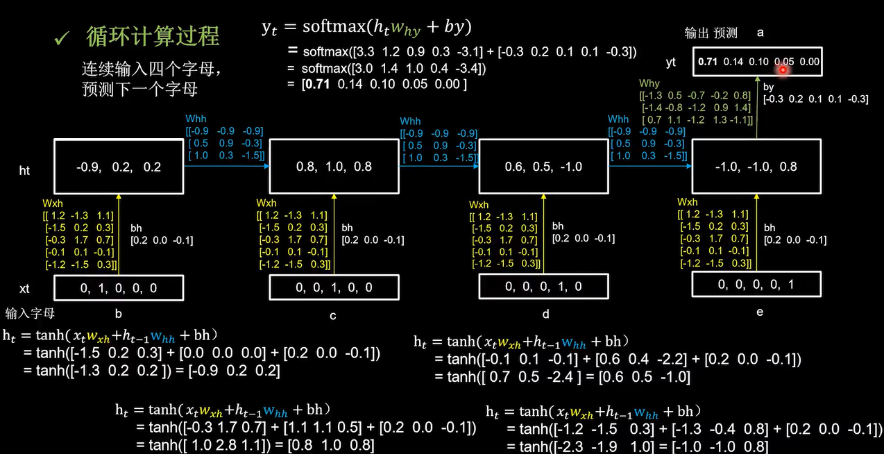
百分之70概率是a,预测正确。
字母预测onehot_4pre1
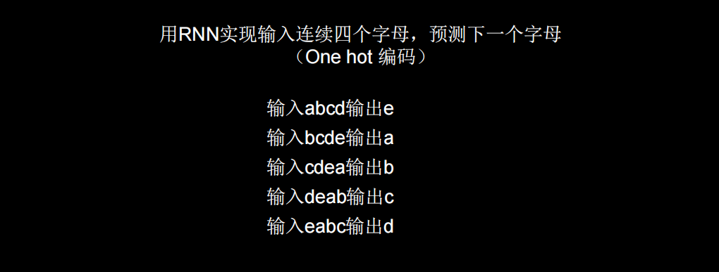
需要修改的地方不多
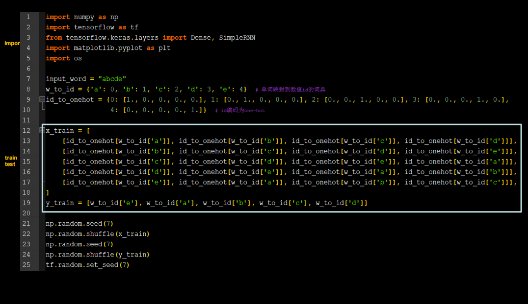
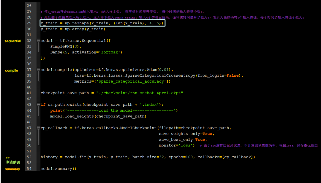
代码如下
import os

import tensorflow as tf
from tensorflow.keras import Sequential
from tensorflow.keras.layers import SimpleRNN, Dense, Dropout
import numpy as np
import matplotlib.pyplot as plt


inputs_word='abcde'
word_id={'a':0,'b':1,'c':2,'d':3,'e':4}
id_onehot={0:[1.,0.,0.,0.,0.],1:[0.,1.,0.,0.,0.],2:[0.,0.,1.,0.,0.],3:[0.,0.,0.,1.,0.],4:[0.,0.,0.,0.,1.]}

x_train=[
    [id_onehot[word_id['a']],id_onehot[word_id['b']],id_onehot[word_id['c']],id_onehot[word_id['d']]],
    [id_onehot[word_id['b']],id_onehot[word_id['c']],id_onehot[word_id['d']],id_onehot[word_id['e']]],
    [id_onehot[word_id['c']],id_onehot[word_id['d']],id_onehot[word_id['e']],id_onehot[word_id['a']]],
    [id_onehot[word_id['d']],id_onehot[word_id['e']],id_onehot[word_id['a']],id_onehot[word_id['b']]],
    [id_onehot[word_id['e']],id_onehot[word_id['a']],id_onehot[word_id['b']],id_onehot[word_id['c']]]
]
# y_train=[id_onehot[word_id['e']],id_onehot[word_id['a']],id_onehot[word_id['b']],id_onehot[word_id['c']],id_onehot[word_id['d']]] #错的
y_train=[word_id['e'],word_id['a'],word_id['b'],word_id['c'],word_id['d']]
# x_train=np.array(x_train)
# y_train=np.array(y_train)
# print(x_train.shape)  # (4, 4, 5)
# print(y_train.shape)  # (4, 5)
np.random.seed(7)
np.random.shuffle(x_train)
np.random.seed(7)
np.random.shuffle(y_train)
tf.random.set_seed(7)


x_train=np.reshape(x_train,[len(x_train),4,5])
y_train=np.array(y_train)


model=Sequential([
    SimpleRNN(3),
    Dense(units=5,activation='softmax')
])

model.compile(tf.keras.optimizers.Adam(0.01),loss=tf.keras.losses.SparseCategoricalCrossentropy(from_logits=False),
              metrics=['sparse_categorical_accuracy'])

checkpoint_path="./checkpoint/rnn_ont4pre1.ckpt"
if os.path.exists(checkpoint_path+'.index'):
    print('---------------------load  model-------------------------')
    model.load_weights(checkpoint_path)

cp_callback = tf.keras.callbacks.ModelCheckpoint(checkpoint_path,monitor='loss',
                                                 save_best_only=True,save_weights_only=True)

history=model.fit(x_train,y_train,batch_size=32,epochs=100,callbacks=[cp_callback])
model.summary()

acc = history.history['sparse_categorical_accuracy']
loss = history.history['loss']

plt.subplot(1, 2, 1)
plt.plot(acc, label='Training Accuracy')
plt.title('Training Accuracy')
plt.legend()

plt.subplot(1, 2, 2)
plt.plot(loss, label='Training Loss')
plt.title('Training Loss')
plt.legend()
plt.show()

input_s=int(input("Enter the number "))
for i in range(input_s):
    x=input('输入一串字符串,长度为4')
    x_pre=[id_onehot[word_id[a]] for a in x]
    x_pre=np.reshape(x_pre,(1,4,5))
    y_pred=model.predict(x_pre)
    y_pred=np.argmax(y_pred,axis=1)
    y=int(y_pred)
    print(inputs_word[y])
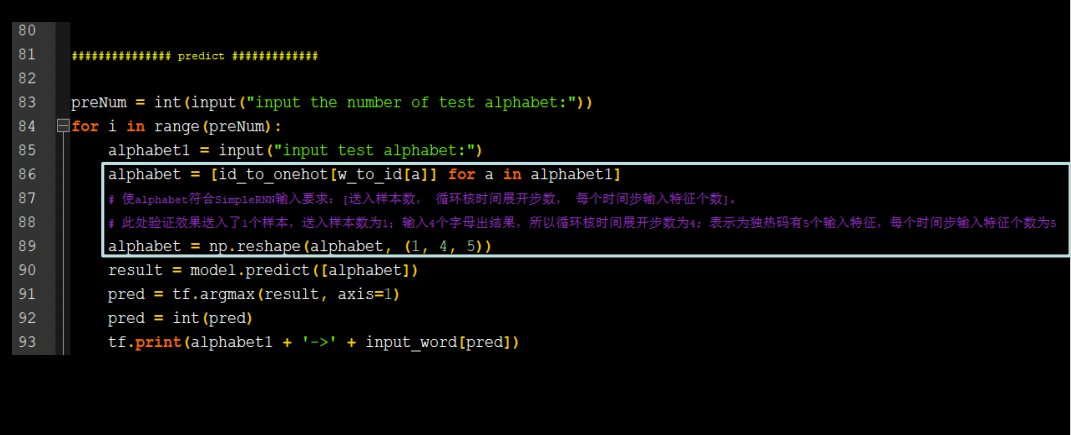
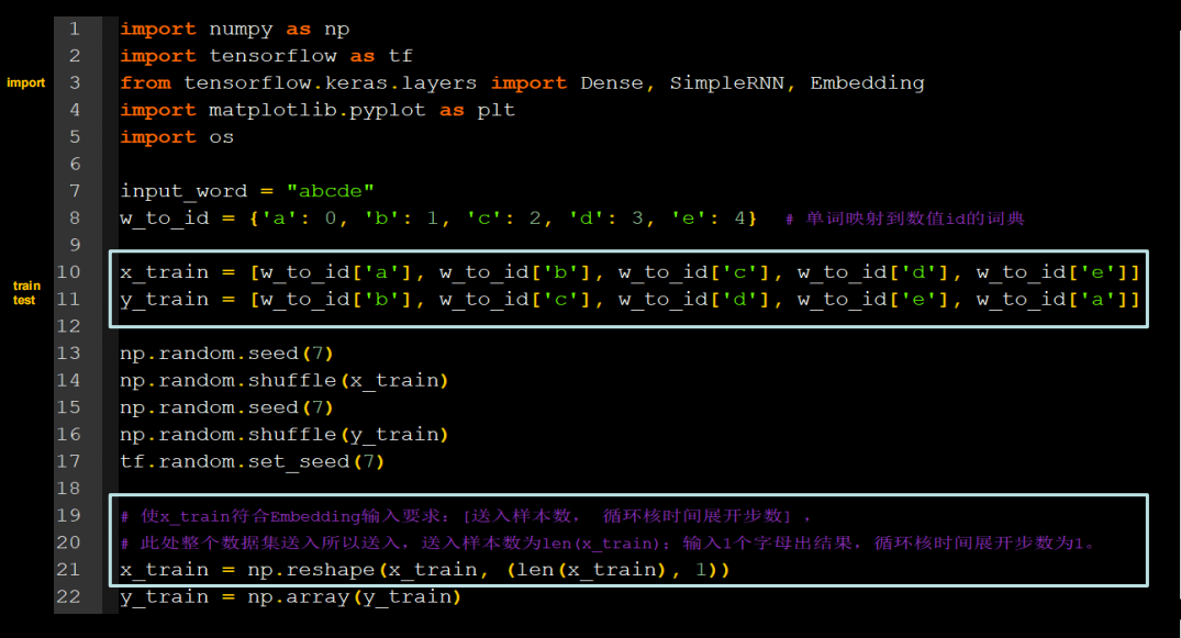
Embedding编码
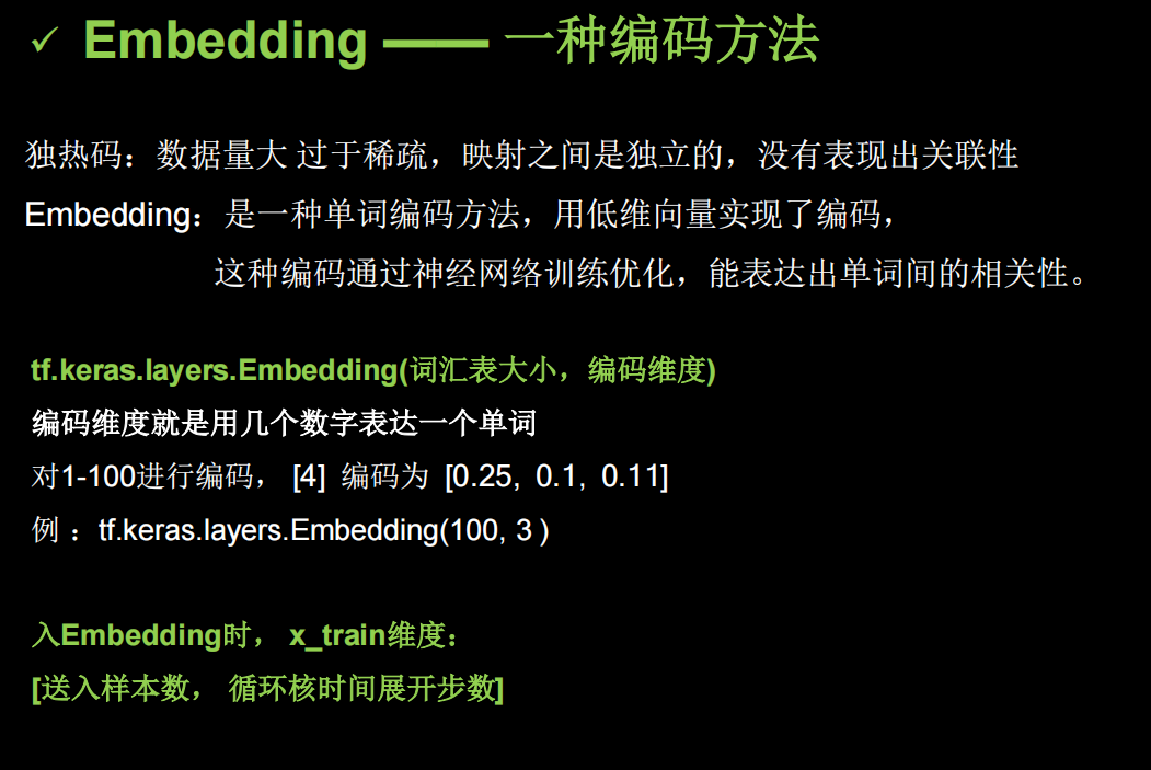
用RNN实现输入一个字母,预测下一个字母(Embedding 编码)
全部代码如下
import os
import tensorflow as tf
from tensorflow.keras import Sequential
from tensorflow.keras.layers import SimpleRNN, Dense, Dropout,Embedding
import numpy as np
import matplotlib.pyplot as plt
inputs_word='abcde'
word_id={'a':0,'b':1,'c':2,'d':3,'e':4}
x_train=[word_id['a'],word_id['b'],word_id['c'],word_id['d'],word_id['e']]
y_train=[word_id['b'],word_id['c'],word_id['d'],word_id['e'],word_id['a']]
np.random.seed(7)
np.random.shuffle(x_train)
np.random.seed(7)
np.random.shuffle(y_train)
tf.random.set_seed(7)
x_train=np.reshape(x_train,[len(x_train),1])
y_train=np.array(y_train)
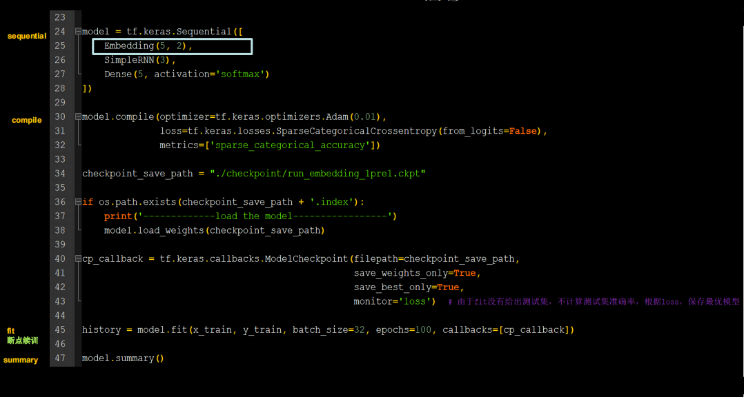
model=Sequential([
Embedding(5,3), # (5,2),(5,5),(5,4) 第一个数是字典长度,即输入数据最大下标+1。第二个数可以随意,表示嵌入的维度
SimpleRNN(3),
Dense(units=5,activation='softmax')
])
model.compile(tf.keras.optimizers.Adam(0.01),loss=tf.keras.losses.SparseCategoricalCrossentropy(from_logits=False),
metrics=['sparse_categorical_accuracy'])
checkpoint_path="./checkpoint/rnn_Embed1pre1.ckpt"
if os.path.exists(checkpoint_path+'.index'):
print('---------------------load model-------------------------')
model.load_weights(checkpoint_path)
cp_callback = tf.keras.callbacks.ModelCheckpoint(checkpoint_path,monitor='loss',
save_best_only=True,save_weights_only=True)
history=model.fit(x_train,y_train,batch_size=32,epochs=100,callbacks=[cp_callback])
model.summary()
acc = history.history['sparse_categorical_accuracy']
loss = history.history['loss']
plt.subplot(1, 2, 1)
plt.plot(acc, label='Training Accuracy')
plt.title('Training Accuracy')
plt.legend()
plt.subplot(1, 2, 2)
plt.plot(loss, label='Training Loss')
plt.title('Training Loss')
plt.legend()
plt.show()
input_s=int(input("Enter the number "))
for i in range(input_s):
al=input('输入一个字符串')
x=word_id[al]
x=np.reshape(x,(1,1))
y=model.predict(x)
y=np.argmax(y,axis=1)
y=int(y)
print(al+'--->'+inputs_word[y])
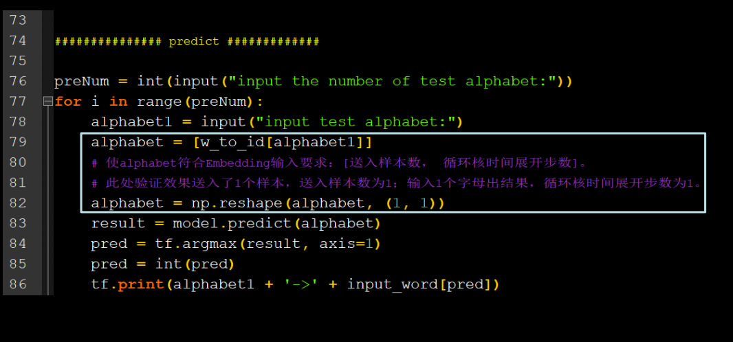
用Embedding预测4pre1
用RNN实现输入连续四个字母,预测下一个字母(Embedding 编码)
增加了数据范围
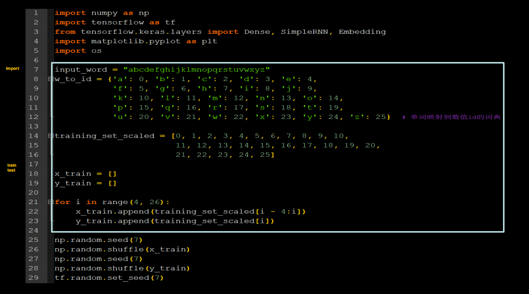
代码如下
import os
import tensorflow as tf
from tensorflow.keras import Sequential
from tensorflow.keras.layers import SimpleRNN, Dense, Dropout,Embedding
import numpy as np
import matplotlib.pyplot as plt
input_word = "abcdefghijklmnopqrstuvwxyz"
w_to_id = {'a': 0, 'b': 1, 'c': 2, 'd': 3, 'e': 4,
'f': 5, 'g': 6, 'h': 7, 'i': 8, 'j': 9,
'k': 10, 'l': 11, 'm': 12, 'n': 13, 'o': 14,
'p': 15, 'q': 16, 'r': 17, 's': 18, 't': 19,
'u': 20, 'v': 21, 'w': 22, 'x': 23, 'y': 24, 'z': 25} # 单词映射到数值id的词典
training_set_scaled = [0, 1, 2, 3, 4, 5, 6, 7, 8, 9, 10,
11, 12, 13, 14, 15, 16, 17, 18, 19, 20,
21, 22, 23, 24, 25]
x_train=[]
y_train=[]
for i in range(4,26):
x_train.append(training_set_scaled[i-4:i])
y_train.append(training_set_scaled[i])
np.random.seed(7)
np.random.shuffle(x_train)
np.random.seed(7)
np.random.shuffle(y_train)
tf.random.set_seed(7)
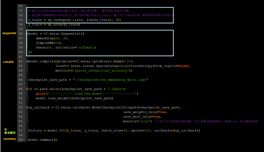
x_train=np.reshape(x_train,[len(x_train),4])
y_train=np.array(y_train)
model=Sequential([
Embedding(26,3),
SimpleRNN(10),
Dense(units=26,activation='softmax')
])
model.compile(tf.keras.optimizers.Adam(0.01),loss=tf.keras.losses.SparseCategoricalCrossentropy(from_logits=False),
metrics=['sparse_categorical_accuracy'])
checkpoint_path="./checkpoint/rnn_Embed4pre4.ckpt"
if os.path.exists(checkpoint_path+'.index'):
print('---------------------load model-------------------------')
model.load_weights(checkpoint_path)
cp_callback = tf.keras.callbacks.ModelCheckpoint(checkpoint_path,monitor='loss',
save_best_only=True,save_weights_only=True)
history=model.fit(x_train,y_train,batch_size=32,epochs=100,callbacks=[cp_callback])
model.summary()
acc = history.history['sparse_categorical_accuracy']
loss = history.history['loss']
plt.subplot(1, 2, 1)
plt.plot(acc, label='Training Accuracy')
plt.title('Training Accuracy')
plt.legend()
plt.subplot(1, 2, 2)
plt.plot(loss, label='Training Loss')
plt.title('Training Loss')
plt.legend()
plt.show()
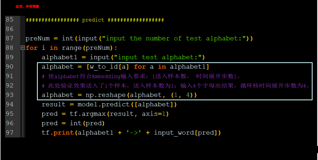
input_s=int(input("Enter the number "))
for i in range(input_s):
x=input('输入一串字符串,长度为4')
x_pre=[w_to_id[a] for a in x]
x_pre=np.reshape(x_pre,(1,4))
y_pred=model.predict(x_pre)
y_pred=np.argmax(y_pred,axis=1)
y=int(y_pred)
print(input_word[y])
RNN实现股票预测
Minmax Scaler不能处理特征只有一维的数据,需要.reshape(-1,1),文件下载
import os
from sklearn.metrics import mean_squared_error, mean_absolute_error
import tensorflow as tf
import numpy as np
import matplotlib.pyplot as plt
import pandas as pd
from sklearn.preprocessing import MinMaxScaler
from tensorflow.keras.layers import Dense, Dropout,SimpleRNN
from tensorflow.keras import Sequential
import math

df=pd.read_csv('./class6/SH600519.csv')

x_train=df.iloc[:2426-300,2].values.reshape(-1,1)
x_test=df.iloc[2426-300:,2].values.reshape(-1,1)

scaler=MinMaxScaler(feature_range=(0,1))
x_train=scaler.fit_transform(x_train)
x_test=scaler.transform(x_test)

x_data_train=[]
y_data_train=[]

for i in range(60,len(x_train)):
    ss=x_train[i-60:i,0]
    # sss=x_train[i-60:i]
    x_data_train.append(ss)
    xx=x_train[i,0]
    y_data_train.append(xx)

x_data_test=[]
y_data_test=[]
for i in range(60,len(x_test)):
    ss=x_test[i-60:i,0]
    x_data_test.append(ss)
    xx=x_test[i,0]
    y_data_test.append(xx)


np.random.seed(33)
np.random.shuffle(x_data_train)
np.random.seed(33)
np.random.shuffle(y_data_train)

x_data_train,y_data_train=np.array(x_data_train),np.array(y_data_train)
x_data_test,y_data_test=np.array(x_data_test),np.array(y_data_test)
x_data_train=np.reshape(x_data_train,(len(x_data_train),60,1))
x_data_test=np.reshape(x_data_test,(len(x_data_test),60,1))

model=Sequential(
    [
        SimpleRNN(units=80,return_sequences=True),
        Dropout(0.2),
        SimpleRNN(units=100),
        Dropout(0.2),
        Dense(1)
    ]
)

model.compile(optimizer='adam',loss='mean_squared_error')

checkpoint_path='./checkpoint/rnn_maotai.ckpt'
if os.path.exists(checkpoint_path+'.index'):
    print('------------------load model -----------------')
    model.load_weights(checkpoint_path)

cp_callback = tf.keras.callbacks.ModelCheckpoint(checkpoint_path,save_best_only=True,save_weights_only=True)

history=model.fit(x_data_train,y_data_train,epochs=50,callbacks=[cp_callback],validation_data=(x_data_test,y_data_test),
                  batch_size=64,validation_freq=1)
model.summary()


loss = history.history['loss']
val_loss = history.history['val_loss']
plt.plot(loss, label='Training Loss')
plt.plot(val_loss, label='Validation Loss')
plt.title('Training and Validation Loss')
plt.legend()
plt.show()

y_pred = model.predict(x_data_test)
y_pred = scaler.inverse_transform(y_pred)

y_true=scaler.inverse_transform(x_test[60:])

plt.plot(y_true, color='red', label='MaoTai Stock Price')
plt.plot(y_pred, color='blue', label='Predicted MaoTai Stock Price')
plt.title('MaoTai Stock Price Prediction')
plt.xlabel('Time')
plt.ylabel('MaoTai Stock Price')
plt.legend()
plt.show()

mse = mean_squared_error(y_pred, y_true)
rmse = math.sqrt(mean_squared_error(y_pred, y_true))
mae = mean_absolute_error(y_pred, y_true)
print('均方误差: %.6f' % mse)
print('均方根误差: %.6f' % rmse)
print('平均绝对误差: %.6f' % mae)
使用LSTM实现股票预测
当序列长度过长时,RNN的表现并不理想,能不能让网络记忆一个很长序列
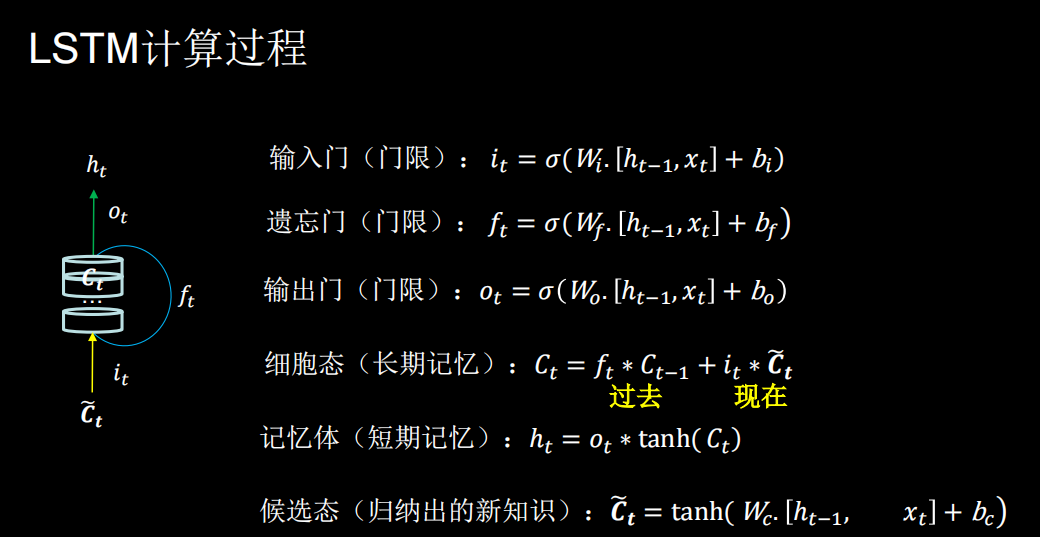
tf中LSTM代码如下
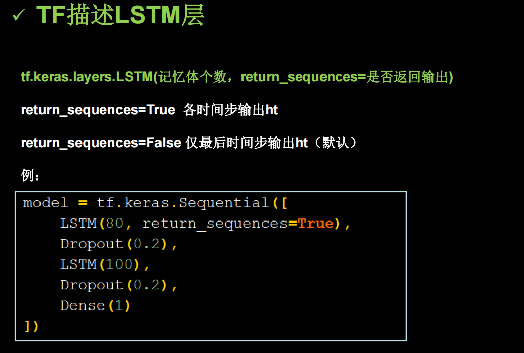
需要改动的只有model里面,其他和上一个代码完全相同
import os
from sklearn.metrics import mean_squared_error, mean_absolute_error
import tensorflow as tf
import numpy as np
import matplotlib.pyplot as plt
import pandas as pd
from sklearn.preprocessing import MinMaxScaler
from tensorflow.keras.layers import Dense, Dropout, SimpleRNN,LSTM
from tensorflow.keras import Sequential
import math

df = pd.read_csv('./class6/SH600519.csv')

x_train = df.iloc[:2426 - 300, 2].values.reshape(-1, 1)
x_test = df.iloc[2426 - 300:, 2].values.reshape(-1, 1)

scaler = MinMaxScaler(feature_range=(0, 1))
x_train = scaler.fit_transform(x_train)
x_test = scaler.transform(x_test)

x_data_train = []
y_data_train = []

for i in range(60, len(x_train)):
    ss = x_train[i - 60:i, 0]
    # sss=x_train[i-60:i]
    x_data_train.append(ss)
    xx = x_train[i, 0]
    y_data_train.append(xx)

x_data_test = []
y_data_test = []
for i in range(60, len(x_test)):
    ss = x_test[i - 60:i, 0]
    x_data_test.append(ss)
    xx = x_test[i, 0]
    y_data_test.append(xx)

np.random.seed(33)
np.random.shuffle(x_data_train)
np.random.seed(33)
np.random.shuffle(y_data_train)

x_data_train, y_data_train = np.array(x_data_train), np.array(y_data_train)
x_data_test, y_data_test = np.array(x_data_test), np.array(y_data_test)
x_data_train = np.reshape(x_data_train, (len(x_data_train), 60, 1))
x_data_test = np.reshape(x_data_test, (len(x_data_test), 60, 1))

model = Sequential(
    [
        LSTM(80,return_sequences=True),
        Dropout(0.2),
        LSTM(100),
        Dropout(0.2),
        Dense(1)
    ]
)

model.compile(optimizer='adam', loss='mean_squared_error')

checkpoint_path = './checkpoint/LSTM_maotai.ckpt'
if os.path.exists(checkpoint_path + '.index'):
    print('------------------load model -----------------')
    model.load_weights(checkpoint_path)

cp_callback = tf.keras.callbacks.ModelCheckpoint(checkpoint_path, save_best_only=True, save_weights_only=True)

history = model.fit(x_data_train, y_data_train, epochs=50, callbacks=[cp_callback],
                    validation_data=(x_data_test, y_data_test),
                    batch_size=64, validation_freq=1)
model.summary()

loss = history.history['loss']
val_loss = history.history['val_loss']
plt.plot(loss, label='Training Loss')
plt.plot(val_loss, label='Validation Loss')
plt.title('Training and Validation Loss')
plt.legend()
plt.show()

y_pred = model.predict(x_data_test)
y_pred = scaler.inverse_transform(y_pred)

y_true = scaler.inverse_transform(x_test[60:])

plt.plot(y_true, color='red', label='MaoTai Stock Price')
plt.plot(y_pred, color='blue', label='Predicted MaoTai Stock Price')
plt.title('MaoTai Stock Price Prediction')
plt.xlabel('Time')
plt.ylabel('MaoTai Stock Price')
plt.legend()
plt.show()

mse = mean_squared_error(y_pred, y_true)
rmse = math.sqrt(mean_squared_error(y_pred, y_true))
mae = mean_absolute_error(y_pred, y_true)
print('均方误差: %.6f' % mse)
print('均方根误差: %.6f' % rmse)
print('平均绝对误差: %.6f' % mae)
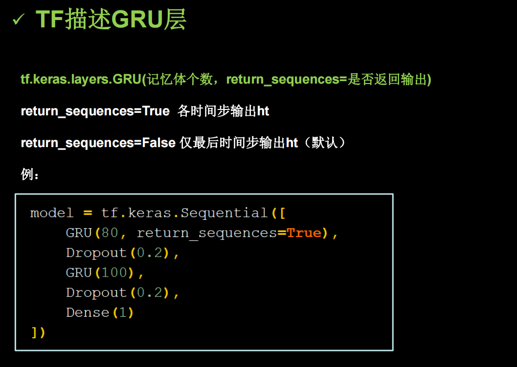
使用GRU实现股票预测
2014提出的GRU简化了LSTM网络
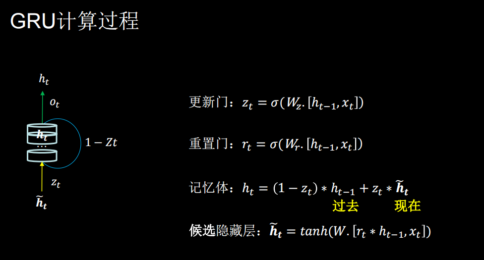
TF中也提供了函数实现GRU
import os
from sklearn.metrics import mean_squared_error, mean_absolute_error
import tensorflow as tf
import numpy as np
import matplotlib.pyplot as plt
import pandas as pd
from sklearn.preprocessing import MinMaxScaler
from tensorflow.keras.layers import Dense, Dropout, SimpleRNN,LSTM,GRU
from tensorflow.keras import Sequential
import math

df = pd.read_csv('./class6/SH600519.csv')

x_train = df.iloc[:2426 - 300, 2].values.reshape(-1, 1)
x_test = df.iloc[2426 - 300:, 2].values.reshape(-1, 1)

scaler = MinMaxScaler(feature_range=(0, 1))
x_train = scaler.fit_transform(x_train)
x_test = scaler.transform(x_test)

x_data_train = []
y_data_train = []

for i in range(60, len(x_train)):
    ss = x_train[i - 60:i, 0]
    # sss=x_train[i-60:i]
    x_data_train.append(ss)
    xx = x_train[i, 0]
    y_data_train.append(xx)

x_data_test = []
y_data_test = []
for i in range(60, len(x_test)):
    ss = x_test[i - 60:i, 0]
    x_data_test.append(ss)
    xx = x_test[i, 0]
    y_data_test.append(xx)

np.random.seed(33)
np.random.shuffle(x_data_train)
np.random.seed(33)
np.random.shuffle(y_data_train)

x_data_train, y_data_train = np.array(x_data_train), np.array(y_data_train)
x_data_test, y_data_test = np.array(x_data_test), np.array(y_data_test)
x_data_train = np.reshape(x_data_train, (len(x_data_train), 60, 1))
x_data_test = np.reshape(x_data_test, (len(x_data_test), 60, 1))

model = Sequential(
    [
        GRU(80,return_sequences=True),
        Dropout(0.2),
        GRU(100),
        Dropout(0.2),
        Dense(1)
    ]
)

model.compile(optimizer='adam', loss='mean_squared_error')

checkpoint_path = './checkpoint/GRU_maotai.ckpt'
if os.path.exists(checkpoint_path + '.index'):
    print('------------------load model -----------------')
    model.load_weights(checkpoint_path)

cp_callback = tf.keras.callbacks.ModelCheckpoint(checkpoint_path, save_best_only=True, save_weights_only=True)

history = model.fit(x_data_train, y_data_train, epochs=50, callbacks=[cp_callback],
                    validation_data=(x_data_test, y_data_test),
                    batch_size=64, validation_freq=1)
model.summary()

loss = history.history['loss']
val_loss = history.history['val_loss']
plt.plot(loss, label='Training Loss')
plt.plot(val_loss, label='Validation Loss')
plt.title('Training and Validation Loss')
plt.legend()
plt.show()

y_pred = model.predict(x_data_test)
y_pred = scaler.inverse_transform(y_pred)

y_true = scaler.inverse_transform(x_test[60:])

plt.plot(y_true, color='red', label='MaoTai Stock Price')
plt.plot(y_pred, color='blue', label='Predicted MaoTai Stock Price')
plt.title('MaoTai Stock Price Prediction')
plt.xlabel('Time')
plt.ylabel('MaoTai Stock Price')
plt.legend()
plt.show()

mse = mean_squared_error(y_pred, y_true)
rmse = math.sqrt(mean_squared_error(y_pred, y_true))
mae = mean_absolute_error(y_pred, y_true)
print('均方误差: %.6f' % mse)
print('均方根误差: %.6f' % rmse)
print('平均绝对误差: %.6f' % mae)