关键点:
1.理解图结构的形式
2.如何使用邻接矩阵实现其图结构形式
3.GCN卷积是如何实现节点特征更新的
核心公式:
特征提取:
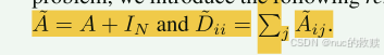
A尖换元后:
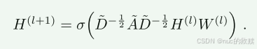
传播规则:
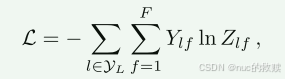
loss:
1.数据处理有价值的代码:
对labels
列,进行
one hot
编码。
就是将 有限个 不管是什么类型的数据,用
不同顺序的01数表示出来。
def encode_onehot(labels):
classes = set(labels)
//for i,c in enumerate(classes):
// print(i,c)
classes_dict = {c: np.identity(len(classes))[i, :] for i, c in
enumerate(classes)}
//print(classes_dict)
labels_onehot = np.array(list(map(classes_dict.get, labels)),
dtype=np.int32)
return labels_onehot
labels = encode_onehot(idx_features_labels[:, -1])
还能把1的位置转换成一维的
labels = torch.LongTensor(np.where(labels)[1])
同理,给了很杂乱的
结点input,可以用
dic去编码。{原label:现label}
idx = np.array(idx_features_labels[:, 0], dtype=np.int32)
idx_map = {j: i for i, j in enumerate(idx)}
随后用编码过的节点,去
编码边
edges_unordered = 边数据
edges = np.array(list(map(idx_map.get, edges_unordered.flatten())),dtype=np.int32).reshape(edges_unordered.shape)
给了边 构建
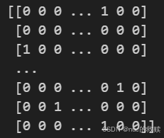
邻接矩阵且为稀疏矩阵
adj = sp.coo_matrix((np.ones(edges.shape[0]), (edges[:, 0], edges[:, 1])),
shape=(labels.shape[0], labels.shape[0]),
dtype=np.float32)
print(adj)
计算转置矩阵将
有向图转化为无向图
adj = adj + adj.T.multiply(adj.T > adj) - adj.multiply(adj.T > adj)
归一化函数
def normalize(mx):
rowsum = np.array(mx.sum(1)) #矩阵行求和
r_inv = np.power(rowsum, -1).flatten() ##求和的倒数
r_inv[np.isinf(r_inv)] = 0.#由于原本为0的数求倒数后可能会产生极大值,这里设置极大值为0
r_mat_inv = sp.diags(r_inv) ##构造对角线矩阵
mx = r_mat_inv.dot(mx)
return mx
adj = normalize(adj + sp.eye(adj.shape[0])) #对应论文中公式,加上了I矩阵
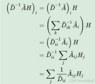
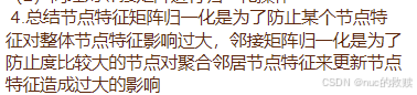
这种归一化方式,将不再单单地对领域节特征点取平均,它不仅
考虑了节点i ii的
度,也考虑了邻接节点j jj的度,
当邻居节点 j jj
度数较大时,它在聚合时贡献地会更少
2.缺点:
第一,GCN需要将整个图放到内存和显存,这将非常耗内存和显存,处理不了大图;
第二,GCN在训练时需要知道整个图的结构信息(包括待预测的节点), 这在现实某些任务中也不能实现(比如用今天训练的图模型预测明天的数据,那么明天的节点是拿不到的)。


![[MySQL]02 存储引擎与索引,锁机制,SQL优化](https://i-blog.csdnimg.cn/direct/4a7e96cd8fb34e92ae4184d7f333b0ef.png)