日期

心得

越往后，越看不懂，只能说是有了解到如何去训练模型代码，对于模型代码该如何去保存，如何通过网络模型去训练。只能一步步来，目前来说是推进度，等后面全部有了认知，再回来重新学习

昇思MindSpore 基础入门学习 模型训练 (AI 代码解析)

模型训练

模型训练一般分为四个步骤：

1. 构建数据集。
2. 定义神经网络模型。
3. 定义超参、损失函数及优化器。
4. 输入数据集进行训练与评估。

现在我们有了数据集和模型后，可以进行模型的训练与评估。

构建数据集

首先从数据集 Dataset加载代码，构建数据集。

import mindspore
from mindspore import nn
from mindspore.dataset import vision, transforms
from mindspore.dataset import MnistDataset

# Download data from open datasets
from download import download

url = "https://mindspore-website.obs.cn-north-4.myhuaweicloud.com/" \
      "notebook/datasets/MNIST_Data.zip"
path = download(url, "./", kind="zip", replace=True)


def datapipe(path, batch_size):
    image_transforms = [
        vision.Rescale(1.0 / 255.0, 0),  # Rescale the image to [0, 1]
        vision.Normalize(mean=(0.1307,), std=(0.3081,)),  # Normalize the image
        vision.HWC2CHW()  # Convert image from HWC format to CHW format
    ]
    label_transform = transforms.TypeCast(mindspore.int32)  # Cast label to int32

    dataset = MnistDataset(path)  # Load MNIST dataset
    dataset = dataset.map(image_transforms, 'image')  # Apply image transformations
    dataset = dataset.map(label_transform, 'label')  # Apply label transformation
    dataset = dataset.batch(batch_size)  # Batch the dataset
    return dataset

train_dataset = datapipe('MNIST_Data/train', batch_size=64)  # Create training dataset
test_dataset = datapipe('MNIST_Data/test', batch_size=64)  # Create test dataset

1. 导入模块:
   • mindspore: MindSpore的主模块，用于深度学习模型的构建和训练。
   • mindspore.nn: 包含神经网络层和损失函数等。
   • mindspore.dataset.vision: 包含图像处理相关的数据增强和变换函数。
   • mindspore.dataset.transforms: 包含数据变换函数。
   • mindspore.dataset.MnistDataset: 用于加载MNIST数据集。
   • download: 用于从指定URL下载数据。
2. 下载数据:
   • url: 存储MNIST数据集的URL。
   • path = download(url, "./", kind="zip", replace=True): 下载并解压数据集到当前目录。
3. **数据处理函数 **datapipe:
   • image_transforms: 一系列图像变换操作，包括重缩放、标准化和格式转换。
     • vision.Rescale(1.0 / 255.0, 0): 将图像像素值从[0, 255]缩放到[0, 1]。
     • vision.Normalize(mean=(0.1307,), std=(0.3081,)): 对图像进行标准化处理。
     • vision.HWC2CHW(): 将图像从高度-宽度-通道(HWC)格式转换为通道-高度-宽度(CHW)格式。
   • label_transform: 将标签数据转换为int32类型。
   • dataset = MnistDataset(path): 加载MNIST数据集。
   • dataset = dataset.map(image_transforms, 'image'): 对图像应用上述变换。
   • dataset = dataset.map(label_transform, 'label'): 对标签应用类型转换。
   • dataset = dataset.batch(batch_size): 将数据集分批处理。
4. 创建训练和测试数据集:
   • train_dataset = datapipe('MNIST_Data/train', batch_size=64): 创建训练数据集。
   • test_dataset = datapipe('MNIST_Data/test', batch_size=64): 创建测试数据集。

• mindspore.dataset.vision.Rescale: 用于图像像素值的缩放。
• mindspore.dataset.vision.Normalize: 用于图像的标准化处理。
• mindspore.dataset.vision.HWC2CHW: 用于图像格式的转换。
• mindspore.dataset.transforms.TypeCast: 用于数据类型的转换。
• mindspore.dataset.MnistDataset: 用于加载MNIST数据集。
• dataset.map: 用于对数据集中的数据应用指定的变换。
• dataset.batch: 用于将数据集分批处理。

定义神经网络模型
从网络构建中加载代码，构建一个神经网络模型。

class Network(nn.Cell):
    def __init__(self):
        super().__init__()
        self.flatten = nn.Flatten()  # Flatten the input tensor into a 2D matrix
        self.dense_relu_sequential = nn.SequentialCell(
            nn.Dense(28*28, 512),  # Fully connected layer with input size 28*28 and output size 512
            nn.ReLU(),  # Apply ReLU activation function
            nn.Dense(512, 512),  # Another fully connected layer with output size 512
            nn.ReLU(),  # Apply ReLU activation function
            nn.Dense(512, 10)  # Fully connected layer with output size 10 for classification
        )

    def construct(self, x):
        x = self.flatten(x)  # Flatten the input
        logits = self.dense_relu_sequential(x)  # Pass the input through the sequential dense layers with ReLU
        return logits  # Return the output logits

model = Network()  # Instantiate the neural network model

1. **定义网络结构 **Network:
   • 继承自 mindspore.nn.Cell，这是MindSpore中神经网络模块的基类。
   • __init__ 方法定义了网络的层次结构：
     • self.flatten: 一个 Flatten 层，将输入的多维张量展平为二维张量。
     • self.dense_relu_sequential: 一个 SequentialCell 容器，按顺序包含多个层：
       • nn.Dense(28*28, 512): 一个全连接层，将输入张量从28x28（MNIST图像尺寸）展平后变成512维向量。
       • nn.ReLU(): 一个ReLU激活函数，用于引入非线性。
       • nn.Dense(512, 512): 另一个全连接层，输入输出尺寸都是512维。
       • nn.ReLU(): 再次使用ReLU激活函数。
       • nn.Dense(512, 10): 最后的全连接层，输出10个类别的得分（用于分类任务）。
2. construct** 方法**:
   • 定义了前向传播的过程：
     • x = self.flatten(x): 将输入张量展平。
     • logits = self.dense_relu_sequential(x): 将展平后的张量通过定义好的全连接层序列。
3. 实例化模型:
   • model = Network(): 创建 Network 类的实例，也就是我们定义的神经网络模型。

• nn.Cell: MindSpore中所有神经网络模块的基类。
• nn.Flatten: 将输入张量展平成二维张量。
• nn.Dense: 全连接层，参数包括输入和输出的维度。
• nn.ReLU: ReLU激活函数，应用非线性变换。
• nn.SequentialCell: 用于按顺序容纳和执行多个子层。

定义超参、损失函数和优化器

超参

超参（Hyperparameters）是可以调整的参数，可以控制模型训练优化的过程，不同的超参数值可能会影响模型训练和收敛速度。目前深度学习模型多采用批量随机梯度下降算法进行优化，随机梯度下降算法的原理如下：

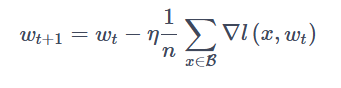
公式中，n𝑛是批量大小（batch size），ηη是学习率（learning rate）。另外，wt𝑤𝑡为训练轮次t𝑡中的权重参数，∇l∇𝑙为损失函数的导数。除了梯度本身，这两个因子直接决定了模型的权重更新，从优化本身来看，它们是影响模型性能收敛最重要的参数。一般会定义以下超参用于训练：

• 训练轮次（epoch）：训练时遍历数据集的次数。
• 批次大小（batch size）：数据集进行分批读取训练，设定每个批次数据的大小。batch size过小，花费时间多，同时梯度震荡严重，不利于收敛；batch size过大，不同batch的梯度方向没有任何变化，容易陷入局部极小值，因此需要选择合适的batch size，可以有效提高模型精度、全局收敛。
• 学习率（learning rate）：如果学习率偏小，会导致收敛的速度变慢，如果学习率偏大，则可能会导致训练不收敛等不可预测的结果。梯度下降法被广泛应用在最小化模型误差的参数优化算法上。梯度下降法通过多次迭代，并在每一步中最小化损失函数来预估模型的参数。学习率就是在迭代过程中，会控制模型的学习进度。

epochs = 3  # Number of complete passes through the training dataset
batch_size = 64  # Number of samples per gradient update
learning_rate = 1e-2  # Step size at each iteration while moving toward a minimum of a loss function

1. epochs:
   • 定义了训练过程中数据集被完整遍历的次数。在每个epoch中，模型会看到整个训练数据集一次。增加epoch的数量可能会提高模型的性能，但同时也增加了过拟合的风险。
2. batch_size:
   • 定义了每次梯度更新时使用的样本数量。较大的batch size可以提供更稳定的梯度估计，但可能会增加内存需求。较小的batch size可能导致训练过程更加不稳定，但有时可以提供更好的泛化性能。
3. learning_rate:
   • 定义了优化算法（如梯度下降）在每次更新模型参数时的步长。学习率太大可能导致模型无法收敛，而学习率太小可能导致训练过程非常缓慢。选择合适的学习率是训练过程中的一个重要步骤。

这些参数通常需要根据具体问题和数据集进行调整，以达到最佳的训练效果。

损失函数
损失函数（loss function）用于评估模型的预测值（logits）和目标值（targets）之间的误差。训练模型时，随机初始化的神经网络模型开始时会预测出错误的结果。损失函数会评估预测结果与目标值的相异程度，模型训练的目标即为降低损失函数求得的误差。
常见的损失函数包括用于回归任务的nn.MSELoss（均方误差）和用于分类的nn.NLLLoss（负对数似然）等。 nn.CrossEntropyLoss 结合了nn.LogSoftmax和nn.NLLLoss，可以对logits 进行归一化并计算预测误差。

loss_fn = nn.CrossEntropyLoss()  # Define the loss function as cross-entropy loss

• loss_fn:
  • 定义了损失函数，用于衡量模型输出（预测值）与实际标签之间的差距。在神经网络的训练过程中，损失函数的输出值用于指导模型参数的更新，以使预测结果更加准确。
• nn.CrossEntropyLoss():
  • Cross-Entropy Loss（交叉熵损失）是一种常用于分类任务的损失函数，尤其适用于多分类问题。它结合了 softmax 和 negative log likelihood，即先将模型的输出通过 softmax 函数转化为概率分布，然后计算实际标签与预测概率分布之间的交叉熵。
  • 在多分类任务中，交叉熵损失能够有效地衡量预测的概率分布与真实分布的差异，从而帮助模型在训练过程中调整参数，提升分类准确率。

• nn.CrossEntropyLoss:
  • 这是MindSpore中用于多分类任务的损失函数，适用于模型的输出是未归一化的得分（logits）形式。通过将logits输入到 CrossEntropyLoss 中，函数内部会首先计算 softmax，然后计算交叉熵损失。

优化器

模型优化（Optimization）是在每个训练步骤中调整模型参数以减少模型误差的过程。MindSpore提供多种优化算法的实现，称之为优化器（Optimizer）。优化器内部定义了模型的参数优化过程（即梯度如何更新至模型参数），所有优化逻辑都封装在优化器对象中。在这里，我们使用SGD（Stochastic Gradient Descent）优化器。
我们通过model.trainable_params()方法获得模型的可训练参数，并传入学习率超参来初始化优化器。

optimizer = nn.SGD(model.trainable_params(), learning_rate=learning_rate)  # Create an optimizer for training the model

• optimizer:

  • 这个变量是一个优化器对象，它将被用来更新模型的参数以最小化损失函数。优化器根据计算得到的损失通过梯度下降法调整模型权重，以改善模型在训练数据上的表现。

• nn.SGD:

  • nn.SGD 是 “Stochastic Gradient Descent”（随机梯度下降）的缩写。这是最常用的优化算法之一，对于许多机器学习问题而言，它是一个有效的优化方法。
  • 这个函数接受两个主要参数：一是我们想要优化的参数集合，在这里是通过 model.trainable_params() 获得的模型可训练参数；二是学习率 learning_rate。

• model.trainable_params():

  • 这是一个函数，返回模型中所有需要训练（即可以在训练过程中更新的）的参数。在神经网络中，这些通常是权重和偏置参数。

• learning_rate=learning_rate:

  • 这是设置优化器学习率的参数。这里的 learning_rate 是之前定义的变量，它将作为优化器的学习率使用。学习率决定了在每次迭代中参数更新的步长大小。

随机梯度下降通常用于大规模数据集，因为每次迭代时只需要计算小批量数据的梯度，使得训练过程更高效。
在训练过程中，通过微分函数可计算获得参数对应的梯度，将其传入优化器中即可实现参数优化，具体形态如下：
grads = grad_fn(inputs)
optimizer(grads)

训练与评估

设置了超参、损失函数和优化器后，我们就可以循环输入数据来训练模型。一次数据集的完整迭代循环称为一轮（epoch）。每轮执行训练时包括两个步骤：

1. 训练：迭代训练数据集，并尝试收敛到最佳参数。
2. 验证/测试：迭代测试数据集，以检查模型性能是否提升。

接下来我们定义用于训练的train_loop函数和用于测试的test_loop函数。
使用函数式自动微分，需先定义正向函数forward_fn，使用value_and_grad获得微分函数grad_fn。然后，我们将微分函数和优化器的执行封装为train_step函数，接下来循环迭代数据集进行训练即可。

# Define forward function
def forward_fn(data, label):
    logits = model(data)  # Forward pass: compute predicted logits by passing data to the model
    loss = loss_fn(logits, label)  # Compute the loss using the predicted logits and true labels
    return loss, logits  # Return the computed loss and logits

# Get gradient function
grad_fn = mindspore.value_and_grad(forward_fn, None, optimizer.parameters, has_aux=True)
# mindspore.value_and_grad computes both the value of the function and its gradient.
# Arguments:
#   - forward_fn: the function for which we want to compute the gradient
#   - None: no additional arguments for gradient computation
#   - optimizer.parameters: parameters with respect to which gradients are computed
#   - has_aux: indicates that forward_fn returns auxiliary data (logits) along with the loss

# Define function of one-step training
def train_step(data, label):
    (loss, _), grads = grad_fn(data, label)  # Compute loss and gradients for the given data and labels
    optimizer(grads)  # Update model parameters using computed gradients
    return loss  # Return the computed loss

def train_loop(model, dataset):
    size = dataset.get_dataset_size()  # Get the total number of batches in the dataset
    model.set_train()  # Set the model to training mode
    for batch, (data, label) in enumerate(dataset.create_tuple_iterator()):
        loss = train_step(data, label)  # Perform one training step

        if batch % 100 == 0:  # Print loss every 100 batches
            loss, current = loss.asnumpy(), batch  # Convert loss from tensor to numpy for printing
            print(f"loss: {loss:>7f}  [{current:>3d}/{size:>3d}]")  # Print the current loss and batch number

1. forward_fn(data, label):
   • 这是一个前向传播函数，用于计算给定数据 data 和标签 label 的损失值和预测的logits。
   • logits = model(data): 使用模型对输入数据进行前向传播，得到预测的logits。
   • loss = loss_fn(logits, label): 使用交叉熵损失函数计算预测的logits和实际标签之间的损失。
   • 返回损失和logits。
2. grad_fn = mindspore.value_and_grad(forward_fn, None, optimizer.parameters, has_aux=True):
   • 这个函数返回一个新的函数 grad_fn，该函数计算前向函数 forward_fn 的输出值和梯度。
   • grad_fn(data, label): 计算前向函数的损失值和梯度。
   • None: 无需额外的参数。
   • optimizer.parameters: 需要计算梯度的模型参数。
   • has_aux=True: 表示前向函数返回辅助数据（logits）。
3. train_step(data, label):
   • 这是一个训练步骤函数，用于执行一次前向传播、计算梯度并更新模型参数。
   • (loss, _), grads = grad_fn(data, label): 计算损失值和梯度。
   • optimizer(grads): 使用计算得到的梯度更新模型参数。
   • 返回计算得到的损失值。
4. train_loop(model, dataset):
   • 这个函数定义了训练循环，用于迭代整个数据集并训练模型。
   • size = dataset.get_dataset_size(): 获取数据集的总批次数。
   • model.set_train(): 将模型设置为训练模式。
   • for batch, (data, label) in enumerate(dataset.create_tuple_iterator()): 遍历数据集。
     • loss = train_step(data, label): 执行一次训练步骤。
     • if batch % 100 == 0: 每100个批次打印一次损失值。
     • loss.asnumpy(): 将损失值从张量转换为numpy数组，以便打印。
     • print(f"loss: {loss:>7f} [{current:>3d}/{size:>3d}]"): 打印当前批次的损失值和批次编号。

test_loop函数同样需循环遍历数据集，调用模型计算loss和Accuray并返回最终结果。

def test_loop(model, dataset, loss_fn):
    num_batches = dataset.get_dataset_size()  # Get the total number of batches in the dataset
    model.set_train(False)  # Set the model to evaluation mode
    total, test_loss, correct = 0, 0, 0  # Initialize counters for total samples, test loss, and correct predictions
    
    for data, label in dataset.create_tuple_iterator():
        pred = model(data)  # Forward pass: compute predictions by passing data to the model
        total += len(data)  # Update the total number of samples
        test_loss += loss_fn(pred, label).asnumpy()  # Accumulate the test loss, converting it from tensor to numpy
        correct += (pred.argmax(1) == label).asnumpy().sum()  # Count correct predictions, comparing argmax of predictions to labels
    
    test_loss /= num_batches  # Compute the average test loss
    correct /= total  # Compute the accuracy by dividing correct predictions by the total number of samples
    
    print(f"Test: \n Accuracy: {(100 * correct):>0.1f}%, Avg loss: {test_loss:>8f} \n")  # Print the test accuracy and average loss

1. test_loop(model, dataset, loss_fn):
   • 这个函数定义了测试循环，用于在给定数据集上评估模型的性能，包括计算准确率和平均损失。
2. num_batches = dataset.get_dataset_size():
   • 获取数据集的总批次数。
3. model.set_train(False):
   • 设置模型为评估模式。在评估模式下，某些操作（例如 dropout 和 batch normalization）会有不同的行为。
4. total, test_loss, correct = 0, 0, 0:
   • 初始化总样本数、测试损失和正确预测数的计数器。
5. for data, label in dataset.create_tuple_iterator()::
   • 遍历数据集中的每个批次。
6. pred = model(data):
   • 使用模型对输入数据进行前向传播，得到预测结果。
7. total += len(data):
   • 累加当前批次的样本数到总样本数。
8. test_loss += loss_fn(pred, label).asnumpy():
   • 计算当前批次的损失，并累加到总测试损失。将损失从张量转换为 numpy 数组，以便进行数值计算。
9. correct += (pred.argmax(1) == label).asnumpy().sum():
   • 计算当前批次中正确预测的样本数，并累加到总正确预测数。pred.argmax(1) 返回预测结果中每行最大值的索引，这相当于预测的类别。
10. test_loss /= num_batches:

• 计算测试集的平均损失。

11. correct /= total:

• 计算测试集的准确率，即正确预测的样本数除以总样本数。

12. print(f"Test: \n Accuracy: {(100 * correct):>0.1f}%, Avg loss: {test_loss:>8f} \n"):

• 打印测试集的准确率和平均损失，准确率以百分比形式显示，损失保留多位小数。

该代码段用于验证模型在测试集上的性能，计算并输出准确率和平均损失。通过逐批处理数据，累积损失和正确预测的计数，最终计算整体性能指标。

我们将实例化的损失函数和优化器传入train_loop和test_loop中。训练3轮并输出loss和Accuracy，查看性能变化。

loss_fn = nn.CrossEntropyLoss()  # Define the loss function, in this case, Cross Entropy Loss
optimizer = nn.SGD(model.trainable_params(), learning_rate=learning_rate)  # Create an optimizer for training the model using Stochastic Gradient Descent

for t in range(epochs):
    print(f"Epoch {t+1}\n-------------------------------")  # Print the current epoch number
    train_loop(model, train_dataset)  # Call the training loop to train the model for one epoch on the training dataset
    test_loop(model, test_dataset, loss_fn)  # Call the testing loop to evaluate the model on the test dataset
print("Done!")  # Indicate that the training process is complete

1. loss_fn = nn.CrossEntropyLoss():
   • 定义损失函数，这里使用的是交叉熵损失函数。交叉熵损失函数常用于分类任务，它度量了预测的概率分布与真实标签分布之间的距离。
2. optimizer = nn.SGD(model.trainable_params(), learning_rate=learning_rate):
   • 创建一个优化器对象，这里使用的是随机梯度下降（SGD）优化器。它将用于在训练过程中更新模型的可训练参数。
   • model.trainable_params(): 获得模型中所有可以训练的参数。
   • learning_rate=learning_rate: 设置优化器的学习率。学习率决定了每次更新参数时步长的大小。
3. for t in range(epochs)::
   • 用于控制训练的循环次数，即训练的轮数（epochs）。
4. print(f"Epoch {t+1}\n-------------------------------"):
   • 打印当前的训练轮数，帮助跟踪训练进度。
5. train_loop(model, train_dataset):
   • 调用训练循环函数 train_loop，在给定的训练数据集上训练模型一个轮次。
6. test_loop(model, test_dataset, loss_fn):
   • 调用测试循环函数 test_loop，在给定的测试数据集上评估模型的性能，包括计算损失和准确率。
7. print("Done!"):
   • 打印“Done!” 表示训练过程完成。

通过这个代码段，模型将会在指定的训练数据集上进行多轮训练（根据 epochs 的值），并且在每轮训练后对模型在测试数据集上的性能进行评估。这种方式可以帮助追踪模型的训练进展和验证模型的泛化能力。

整体代码

#!/usr/bin/env python
# coding: utf-8

# Import necessary libraries from MindSpore
import mindspore
from mindspore import nn
from mindspore.dataset import vision, transforms
from mindspore.dataset import MnistDataset

# Download data from open datasets
from download import download

# Specify the URL to download the MNIST dataset and the path to save it
url = "https://mindspore-website.obs.cn-north-4.myhuaweicloud.com/" \
      "notebook/datasets/MNIST_Data.zip"
path = download(url, "./", kind="zip", replace=True)

# Function to create and preprocess the dataset
def datapipe(path, batch_size):
    # Define transformations for images
    image_transforms = [
        vision.Rescale(1.0 / 255.0, 0),  # Rescale pixel values to [0, 1]
        vision.normalize(mean=(0.1307,), std=(0.3081,)),  # Normalize with mean and std
        vision.HWC2CHW()  # Change image format from HWC to CHW
    ]
    # Define transformation for labels
    label_transform = transforms.TypeCast(mindspore.int32)

    # Create the dataset
    dataset = MnistDataset(path)
    dataset = dataset.map(image_transforms, 'image')  # Apply image transformations
    dataset = dataset.map(label_transform, 'label')  # Apply label transformation
    dataset = dataset.batch(batch_size)  # Batch the dataset
    return dataset

# Create training and test datasets
train_dataset = datapipe('MNIST_Data/train', batch_size=64)
test_dataset = datapipe('MNIST_Data/test', batch_size=64)

# Define a neural network model
class Network(nn.Cell):
    def __init__(self):
        super().__init__()
        self.flatten = nn.Flatten()  # Flatten the input
        self.dense_relu_sequential = nn.SequentialCell(
            nn.Dense(28*28, 512),  # Fully connected layer with 512 units
            nn.ReLU(),  # ReLU activation
            nn.Dense(512, 512),  # Fully connected layer with 512 units
            nn.ReLU(),  # ReLU activation
            nn.Dense(512, 10)  # Fully connected layer with 10 units for classification
        )

    def construct(self, x):
        x = self.flatten(x)  # Flatten the input
        logits = self.dense_relu_sequential(x)  # Forward pass through the sequential layers
        return logits

# Instantiate the model
model = Network()

# Define hyperparameters
epochs = 3
batch_size = 64
learning_rate = 1e-2

# Define the loss function
loss_fn = nn.CrossEntropyLoss()  # Cross Entropy Loss for classification

# Define the optimizer
optimizer = nn.SGD(model.trainable_params(), learning_rate=learning_rate)  # Stochastic Gradient Descent

# Define forward function
def forward_fn(data, label):
    logits = model(data)  # Forward pass: compute logits
    loss = loss_fn(logits, label)  # Compute loss
    return loss, logits

# Get gradient function
grad_fn = mindspore.value_and_grad(forward_fn, None, optimizer.parameters, has_aux=True)
# mindspore.value_and_grad computes both the value of the function and its gradient.
# Arguments:
#   - forward_fn: the function for which we want to compute the gradient
#   - None: no additional arguments for gradient computation
#   - optimizer.parameters: parameters with respect to which gradients are computed
#   - has_aux: indicates that forward_fn returns auxiliary data (logits) along with the loss

# Define function of one-step training
def train_step(data, label):
    (loss, _), grads = grad_fn(data, label)  # Compute loss and gradients for the given data and labels
    optimizer(grads)  # Update model parameters using computed gradients
    return loss  # Return the computed loss

def train_loop(model, dataset):
    size = dataset.get_dataset_size()  # Get the total number of batches in the dataset
    model.set_train()  # Set the model to training mode
    for batch, (data, label) in enumerate(dataset.create_tuple_iterator()):
        loss = train_step(data, label)  # Perform one training step

        if batch % 100 == 0:  # Print loss every 100 batches
            loss, current = loss.asnumpy(), batch  # Convert loss from tensor to numpy for printing
            print(f"loss: {loss:>7f}  [{current:>3d}/{size:>3d}]")  # Print the current loss and batch number

def test_loop(model, dataset, loss_fn):
    num_batches = dataset.get_dataset_size()  # Get the total number of batches in the dataset
    model.set_train(False)  # Set the model to evaluation mode
    total, test_loss, correct = 0, 0, 0  # Initialize counters for total samples, test loss, and correct predictions
    
    for data, label in dataset.create_tuple_iterator():
        pred = model(data)  # Forward pass: compute predictions by passing data to the model
        total += len(data)  # Update the total number of samples
        test_loss += loss_fn(pred, label).asnumpy()  # Accumulate the test loss, converting it from tensor to numpy
        correct += (pred.argmax(1) == label).asnumpy().sum()  # Count correct predictions, comparing argmax of predictions to labels
    
    test_loss /= num_batches  # Compute the average test loss
    correct /= total  # Compute the accuracy by dividing correct predictions by the total number of samples
    
    print(f"Test: \n Accuracy: {(100 * correct):>0.1f}%, Avg loss: {test_loss:>8f} \n")  # Print the test accuracy and average loss

# Train the model for the specified number of epochs and test it after each epoch
for t in range(epochs):
    print(f"Epoch {t+1}\n-------------------------------")  # Print the current epoch number
    train_loop(model, train_dataset)  # Call the training loop to train the model for one epoch on the training dataset
    test_loop(model, test_dataset, loss_fn)  # Call the testing loop to evaluate the model on the test dataset
print("Done!")  # Indicate that the training process is complete

1. 引入和下载数据集:
   • import mindspore: 导入MindSpore库。
   • from mindspore import nn: 导入神经网络模块。
   • from mindspore.dataset import vision, transforms 和 from mindspore.dataset import MnistDataset: 导入数据集和数据预处理工具。
   • from download import download: 导入下载工具。
   • url** 和 **path: 定义数据集的下载URL和保存路径。
   • path = download(url, "./", kind="zip", replace=True): 下载MNIST数据集。
2. **数据集预处理函数 **datapipe:
   • image_transforms: 定义图像预处理步骤，包括重缩放、归一化和格式转换。
   • label_transform: 定义标签转换步骤。
   • MnistDataset: 加载MNIST数据集。
   • dataset.map(image_transforms, 'image') 和 dataset.map(label_transform, 'label'): 应用图像和标签的预处理。
   • dataset.batch(batch_size): 按批次大小分割数据集。
   • 返回预处理后的数据集。
3. **定义神经网络模型 **Network:
   • nn.Cell: 继承自MindSpore的神经网络模块。
   • self.flatten: 定义flatten层。
   • self.dense_relu_sequential: 使用nn.SequentialCell定义全连接+激活的顺序层。
   • construct: 定义前向传播逻辑。
4. 定义超参数:
   • epochs = 3: 训练轮次。
   • batch_size = 64: 批次大小。
   • learning_rate = 1e-2: 学习率。
5. 定义损失函数和优化器:
   • loss_fn = nn.CrossEntropyLoss(): 定义交叉熵损失函数。
   • optimizer = nn.SGD(model.trainable_params(), learning_rate=learning_rate): 定义随机梯度下降优化器。
6. **定义前向函数 **forward_fn:
   • logits = model(data): 计算logits。
   • loss = loss_fn(logits, label): 计算损失。
   • 返回损失和logits。
7. **获取梯度函数 **grad_fn:
   • grad_fn = mindspore.value_and_grad(forward_fn, None, optimizer.parameters, has_aux=True): 获取前向函数的值和梯度。
8. **定义训练步骤函数 **train_step:
   • (loss, _), grads = grad_fn(data, label): 计算损失和梯度。
   • optimizer(grads): 使用梯度更新模型参数。
   • 返回损失。
9. **定义训练循环 **train_loop:
   • size = dataset.get_dataset_size(): 获取数据集的总批次数。
   • model.set_train(): 设置模型为训练模式。
   • for batch, (data, label) in enumerate(dataset.create_tuple_iterator()): 遍历数据集。
   • loss = train_step(data, label): 执行一次训练步骤。
   • if batch % 100 == 0: 每100个批次打印一次损失。
   • print(f"loss: {loss:>7f} [{current:>3d}/{size:>3d}]"): 打印当前损失和批次编号。
10. **定义测试循环 **test_loop:

• num_batches = dataset.get_dataset_size(): 获取数据集的总批次数。
• model.set_train(False): 设置模型为评估模式。
• total, test_loss, correct = 0, 0, 0: 初始化计数器。
• for data, label in dataset.create_tuple_iterator(): 遍历数据集。
• pred = model(data): 计算预测值。
• total += len(data): 更新总样本数。
• test_loss += loss_fn(pred, label).asnumpy(): 累积测试损失。
• correct += (pred.argmax(1) == label).asnumpy().sum(): 计算正确预测数。
• test_loss /= num_batches: 计算平均测试损失。
• correct /= total: 计算准确率。
• print(f"Test: \n Accuracy: {(100 * correct):>0.1f}%, Avg loss: {test_loss:>8f} \n"): 打印测试集准确率和平均损失。

11. 训练和测试模型:

• for t in range(epochs): 循环训练。
• print(f"Epoch {t+1}\n-------------------------------"): 打印当前训练轮次。
• train_loop(model, train_dataset): 训练模型。
• test_loop(model, test_dataset, loss_fn): 测试模型。
• print("Done!"): 打印训练完成。

该代码段展示了一个完整的深度学习训练流程，包括数据预处理、模型定义、训练和测试。通过循环训练和评估，模型的性能可以逐步得到提升。