Advanced RAG 09：『提示词压缩』技术综述

编者按： 如何最大限度地发挥 LLMs 的强大能力，同时还能控制其推理成本？这是当前业界研究的一个热点课题。

针对这一问题，本期精心选取了一篇关于"提示词压缩"(Prompt Compression)技术的综述文章。正如作者所说，提示词压缩技术的核心目标是压缩向 LLMs 输入的上下文信息，删减非关键内容，保留语义核心，从而在不影响模型表现的前提下，降低推理成本。

文中全面介绍了多种提示词压缩算法的原理和实现细节，包括基于信息熵的Selective Context、基于软提示调优的AutoCompressor、引入数据蒸馏方法的LLMLingua-2、综合利用问题语义的LongLLMLingua等。作者还贴心地附上了代码示例，以便各位读者可以动手实践，加深对算法的理解。

你是否曾因难以处理冗长的提示词而寝食难安，被昂贵的推理成本所困扰？现在，就让我们跟随本文的脚步，开启一场 Prompt Compression 技术的学习之旅吧！也许在了解某个算法时灵感闪现，你就能找到突破瓶颈的金钥匙。

作者 | Florian June

编译 | 岳扬

RAG 方法可能会面临两大挑战：

大语言模型（LLMs）往往有上下文长度（context length）的限制。 这意味着，随着输入文本的长度增长，处理过程不仅变得更加耗时，成本也随之增加。
检索出的上下文未必都能派上用场。 有时，仅有一小部分信息对解答问题有帮助。在某些情形下，为了回答某些特定问题，可能需要整合来自多个文本片段的信息。即便实施了重排序（re-ranking）技术，这一难题依然未能得到解决。

为了解决上述问题，LLM 的提示词压缩技术（Prompt compression）应运而生。从本质上讲，其目的是精炼提示词中的关键信息，使得每个输入的词元（input tokens）都承载更多价值，从而提升模型效率并还能控制成本。这一理念在图 1 的右下角进行了直观展示。

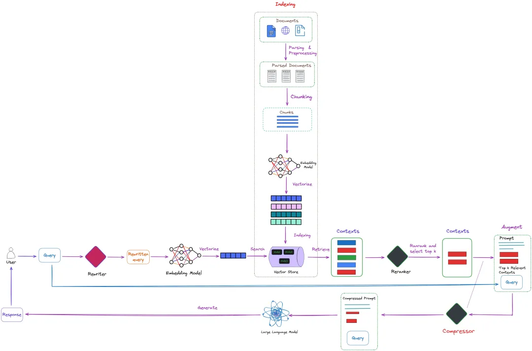
图 1：RAG 架构中的提示词压缩技术（见图右下角）。如紫色虚线标记的部分所示，某些压缩方法能够直接作用于已检索的上下文信息。此图由作者绘制。

如图 1 中紫色虚线标记的部分所示，部分压缩方法可以直接应用于从大语言模型中检索出的上下文信息。

总的来说，提示词压缩方法可以分为四大类：

基于信息熵（information entropy）的方法：例如 Selective Context[1]、LLMLingua[2] 和 LongLLMLingua[3]。这些方法利用小型语言模型来计算原始提示词中每个 token 的自信息（self-information ）（译者注：自信息，又称为惊喜度（surprisal）或信息含量（information content），是信息理论中的核心概念之一。它用来量化某个事件所传达的信息量的大小。）或困惑度（perplexity）。接着删除那些困惑度较低的 token ，实现压缩目的。
基于 soft prompt tuning （译者注：soft prompt tuning 不直接修改模型的权重，而是引入一组可学习的连续向量（通常称为"soft prompts"），这种方法允许模型在不改变其核心结构的情况下适应不同的下游任务，同时保留了模型在预训练阶段学到的一般知识。）的方法：如 AutoCompressor[4] 和 GIST[5]。此类方法需要对大语言模型的参数进行微调，使其适用于特定领域，但不能直接应用于黑盒大语言模型（black-box LLM）。
先进行数据蒸馏，再训练模型生成更易解释的文本摘要：这类方法可以跨不同语言模型迁移，并能应用于无需梯度更新的黑盒大语言模型。代表性的方法包括 LLMLingua-2[6] 和 RECOMP[7]。
基于词元合并（token merging）或词元剪枝（token pruning）的方法：如 ToMe[8] 和 AdapLeR[9]。这些方法通常需要在推理过程中对模型进行微调或生成中间结果。

鉴于第四类方法最初是为了像 ViT 或 BERT 这样的较小模型而提出的，本文将重点介绍前三类方法中代表性算法的原理。

01 Selective Context

1.1 作者的领悟见解

图 2 表明，大语言模型（LLM）即使在缺乏完整上下文或对话历史的情况下，也能对用户的询问做出回应。即便某些相关细节被省略，大语言模型（LLM）依旧能给出用户期望的回答。这或许是因为大语言模型（LLM）能够从上下文信息和预训练阶段积累的知识中推断出缺失的信息。

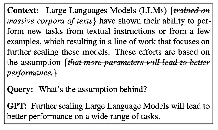
图 2：即便去除了部分非关键信息，大语言模型（LLM）依然能准确作答。来源：《Selective Context》[1]

由此看来，我们可以通过筛选掉非关键信息来优化上下文长度（context length），而不会影响其整体性能。这就是 Selective Context 方法的关键所在。

Selective Context 策略采用小型语言模型（SLM），来计算给定上下文中各个词汇单元（比如句子、短语或词语）的自信息值。然后，基于这些自信息值（self-information）进一步评估各单元的信息含量。通过仅保留自信息值较高的内容，Selective Context 为大语言模型（LLM）提供了更为简洁、高效的 context representation （译者注：经过数学化或模型化文本或对话后的机器可处理的上下文信息）。这一做法不会对其在各种任务中的表现造成负面影响。

1.2 Self-Information 自信息

Selective Context 运用自信息（self-information）来衡量内容的价值。

自信息，又称为惊喜度（surprisal）或信息含量（information content），是信息理论中的核心概念之一。它用来量化某个事件所传达的信息量的大小。具体来说，它是 token 出现概率的负对数形式：

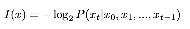
这里，𝐼(𝑥) 代表 token 𝑥 的自信息量，而 𝑃(𝑥) 则指代该 token 的出现概率。

在信息论框架（information theory）下，自信息反映了事件发生时带来的惊喜程度或不确定性程度。那些不常见的事件，由于包含了更多新颖的信息，因而具有较高的自信息值。 相比之下，频繁发生的事件，因其提供的新信息较少，自信息值也就相应较低。

1.3 Algorithm 算法

为了便于阐述其背后的原理，我们不妨一同探究一下其源代码。

首要步骤是配置开发环境，安装必需的 Python 库以及下载 Spacy 模型。

(base) Florian:~ Florian$ conda create -n "selective_context" python=3.10 
(base) Florian:~ Florian$ conda activate selective_context
(selective_context) Florian:~ Florian$ pip install selective-context
(selective_context) Florian:~ Florian$ python -m spacy download en_core_web_sm

安装完成后，版本信息如下：

(selective_context) Florian:~ Florian$ pip list | grep selective
selective-context   0.1.4

测试代码如下所示：

from selective_context import SelectiveContext

sc = SelectiveContext(model_type='gpt2', lang='en')
text = "INTRODUCTION Continual Learning ( CL ) , also known as Lifelong Learning , is a promising learning paradigm to design models that have to learn how to perform multiple tasks across different environments over their lifetime [To uniform the language and enhance the readability of the paper we adopt the unique term continual learning ( CL ) .]. Ideal CL models in the real world should be deal with domain shifts , researchers have recently started to sample tasks from two different datasets . For instance , proposed to train and evaluate a model on Imagenet first and then challenge its performance on the Places365 dataset . considers more scenarios , starting with Imagenet or Places365 , and then moving on to the VOC/CUB/Scenes datasets. Few works propose more advanced scenarios built on top of more than two datasets."
context, reduced_content = sc(text)

# We can also adjust the reduce ratio
# context_ratio, reduced_content_ratio = sc(text, reduce_ratio = 0.5)

初次执行时，系统会自动下载 GPT-2 模型，该模型的文件大小接近 500MB。图 3 呈现了测试代码的具体运行结果。

图 3：Selective Context 算法测试代码运行结果。截图由作者提供。

随后，我们将深入研究 sc(text) 函数。该函数的内部实现代码[10]如下：

class SelectiveContext:
 ...
 ...
 def __call__(self, text: str, reduce_ratio: float = 0.35, reduce_level :str = 'phrase') -> List[str]:
        context = self.beautify_context(text)

        self.mask_ratio = reduce_ratio

        sents = [sent.strip() for sent in re.split(self.sent_tokenize_pattern, context) if sent.strip()]

 # You want the reduce happen at sentence level, phrase level, or token level?
 assert reduce_level in ['sent', 'phrase', 'token'], f"reduce_level should be one of ['sent', 'phrase', 'token'], got {reduce_level}"
        sent_lus, phrase_lus, token_lus = self._lexical_unit(sents)
        lexical_level = {
 'sent': sent_lus,
 'phrase': phrase_lus,
 'token': token_lus
 }

 # context is the reduced context, masked_sents denotes what context has been filtered out
        context, masked_sents = self.self_info_mask(lexical_level[reduce_level].text, lexical_level[reduce_level].self_info, reduce_level)
 return context, masked_sents

这段代码的核心操作分为三个阶段：

首先，计算出上下文中每一个 token 的自信息值。
接着，依据词汇单位（比如短语或句子）整合 token 与其对应的自信息。
最后，采取有选择的方式保留必要的信息上下文，从而达到优化的目的。

第一步：自信息的计算

给定上下文 𝐶=𝑥0,𝑥1,…,𝑥𝑛 ，其中每个 𝑥𝑖 均代表一个 token ，我们可以借助因果语言模型（例如 GPT-2、OPT 或 LLaMA）来求解每个 token 𝑥𝑖 的自信息值：

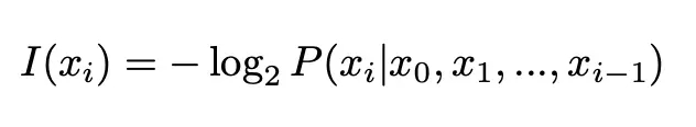
若你选用的是 GPT-2 模型，以下便是实现此计算过程的相应代码片段[11]：

class SelectiveContext:
 ...
 ... 
 def _get_self_info_via_gpt2(self, text: str) -> Tuple[List[str], List[float]]:
 if self.lang == 'en':
            text = f"<|endoftext|>{text}"
 elif self.lang == 'zh':
            text = f"[CLS]{text}"
 with torch.no_grad():
            encoding = self.tokenizer(text, add_special_tokens=False, return_tensors='pt')
            encoding = encoding.to(self.device)
            outputs = self.model(**encoding)
            logits = outputs.logits
            probs = torch.softmax(logits, dim=-1)
            self_info = -torch.log(probs)
 
        input_ids = encoding['input_ids']
        input_ids_expaned = input_ids[:, 1:].unsqueeze(-1)

第二步：整合为词汇单元（Lexical Units）

如果仅仅在 tokens 层面上执行 selective context filtering（译者注：识别和保留那些对当前任务或用户查询最为关键的信息，同时过滤掉不太相关或冗余的部分。），可能会导致最终的上下文失去连贯性。举个例子，原本的数字"2009"在压缩后可能会变成"209"，这样的结果显然不够合理。

鉴于此，除了在 tokens 层面进行筛选外，同时在短语和句子层面上实行过滤策略也是极其重要的。在这里，我们所说的过滤（filtering）基本单位------词汇单元，可以是个别的 token ，也可以是完整的短语或是句子。

那么，怎样才能计算出每个词汇单元 𝑢=(𝑥𝑡,…,𝑥𝑡+𝛼) 的自信息呢？我们可以根据自信息的可加性原则，将组成 u 的每个 token 的自信息相加：

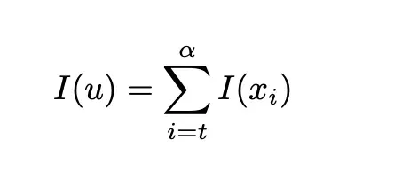
下面是具体的代码实现[12]，为了便于调试，我对部分变量添加了详细的注释：

class SelectiveContext:
 ...
 ...
 def _lexical_unit(self, sents):

 if self.sent_level_self_info:
            sent_self_info = []
            all_noun_phrases = []
            all_noun_phrases_info = []
            all_tokens = []
            all_token_self_info = []

 for sent in sents:
 # print(sent)
                tokens, self_info = self.get_self_information(sent)
 '''
                ipdb> sent
                'INTRODUCTION Continual Learning ( CL ) , also known as Lifelong Learning , is a promising learning paradigm to design models that have to learn how to perform multiple tasks across different environments over their lifetime [To uniform the language and enhance the readability of the paper we adopt the unique term continual learning ( CL ) .].'

                ipdb> tokens
                ['IN', 'TR', 'ODUCT', 'ION', ' Contin', 'ual', ' Learning', ' (', ' CL', ' )', ',', ' also', ' known', ' as', ' Lif', 'elong', ' Learning', ',', ' is', ' a', ' promising', ' learning', ' paradigm', ' to', ' design', ' models', ' that', ' have', ' to', ' learn', ' how', ' to', ' perform', ' multiple', ' tasks', ' across', ' different', ' environments', ' over', ' their', ' lifetime', ' [', 'To', ' uniform', ' the', ' language', ' and', ' enhance', ' the', ' read', 'ability', ' of', ' the', ' paper', ' we', ' adopt', ' the', ' unique', ' term', ' continual', ' learning', ' (', ' CL', ' )', '.', '].']

                ipdb> self_info
                [7.514791011810303, 1.632637619972229, 0.024813441559672356, 0.006853647995740175, 12.09920597076416, 2.1144468784332275, 9.457701683044434, 2.4503376483917236, 10.236454963684082, 0.8689146041870117, 5.269547939300537, 4.641763210296631, 0.22138957679271698, 0.010370315983891487, 10.071824073791504, 0.6905602216720581, 0.01698811538517475, 1.5882389545440674, 0.4495090842247009, 0.45371606945991516, 6.932497978210449, 6.087430477142334, 3.66465425491333, 3.3969509601593018, 7.337691307067871, 5.881226539611816, 1.7340556383132935, 4.599822521209717, 6.482723236083984, 4.045308589935303, 4.762691497802734, 0.21346867084503174, 3.7985599040985107, 4.6389899253845215, 0.33642446994781494, 4.918881416320801, 2.076707601547241, 3.3553669452667236, 5.5081071853637695, 5.625778675079346, 0.7966060638427734, 6.347291946411133, 12.772034645080566, 13.792041778564453, 4.11267614364624, 6.583715915679932, 3.3618998527526855, 8.434362411499023, 1.2423189878463745, 5.8330583572387695, 0.0013973338063806295, 0.3090735077857971, 1.1139129400253296, 4.160390853881836, 3.744772434234619, 7.2841596603393555, 1.4088190793991089, 7.86871337890625, 4.305004596710205, 9.69282341003418, 0.08665203303098679, 1.6127821207046509, 1.6296097040176392, 0.46206924319267273, 3.0398476123809814, 6.892032623291016]
                '''
                sent_self_info.append(np.mean(self_info))

                all_tokens.extend(tokens)
                all_token_self_info.extend(self_info)

                noun_phrases, noun_phrases_info = self._calculate_lexical_unit(tokens, self_info)
 '''
                ipdb> noun_phrases
                ['INTRODUCTION Continual Learning', ' (', ' CL', ' )', ',', ' also', ' known', ' as', ' Lifelong Learning', ',', ' is', ' a promising learning paradigm', ' to', ' design', ' models', ' that', ' have', ' to', ' learn', ' how', ' to', ' perform', ' multiple tasks', ' across', ' different environments', ' over', ' their lifetime', ' [', 'To', ' uniform', ' the language', ' and', ' enhance', ' the readability', ' of', ' the paper', ' we', ' adopt', ' the unique term continual learning', ' (', ' CL', ' )', '.', ']', '.']
 
                ipdb> noun_phrases_info
                [4.692921464797109, 2.4503376483917236, 10.236454963684082, 0.8689146041870117, 5.269547939300537, 4.641763210296631, 0.22138957679271698, 0.010370315983891487, 3.5931241369495788, 1.5882389545440674, 0.4495090842247009, 4.284574694931507, 3.3969509601593018, 7.337691307067871, 5.881226539611816, 1.7340556383132935, 4.599822521209717, 6.482723236083984, 4.045308589935303, 4.762691497802734, 0.21346867084503174, 3.7985599040985107, 2.487707197666168, 4.918881416320801, 2.7160372734069824, 5.5081071853637695, 3.2111923694610596, 6.347291946411133, 12.772034645080566, 13.792041778564453, 5.348196029663086, 3.3618998527526855, 8.434362411499023, 2.3589248929638416, 0.3090735077857971, 2.6371518969535828, 3.744772434234619, 7.2841596603393555, 4.672402499616146, 1.6127821207046509, 1.6296097040176392, 0.46206924319267273, 3.0398476123809814, 3.446016311645508, 3.446016311645508]
                '''

 # We need to add a space before the first noun phrase for every sentence except the first one
 if all_noun_phrases:
                    noun_phrases[0] = f" {noun_phrases[0]}"
                all_noun_phrases.extend(noun_phrases)
                all_noun_phrases_info.extend(noun_phrases_info)
 
 return [
                LexicalUnits('sent', text=sents, self_info=sent_self_info),
                LexicalUnits('phrase', text=all_noun_phrases, self_info=all_noun_phrases_info),
                LexicalUnits('token', text=all_tokens, self_info=all_token_self_info)
 ]

第三步：精选保留信息含量高的上下文

在计算了每个词汇单元的自信息之后，我们面临的问题是如何判断其信息含量。论文介绍了一种创新方法，利用基于百分位数的筛选策略，动态挑选出信息最丰富的内容。这种方法相较于设定固定阈值或仅仅保留前 k 个最高信息量的词汇单元更为灵活有效。

我们的操作流程是先按自信息值（self-information values）从高到低排序所有词汇单元 ，接着计算所有词汇单元自信息值的 p-th percentile （译者注：“p-th percentile” 在统计学中指的是数据分布的一个特定点，在这一点之下包含了总数据中 p% 的数值。举个例子，假设你有一个班级的数学成绩分布，如果某个学生的成绩位于第90百分位（90th percentile），这意味着班上90%的学生的成绩低于或等于他的成绩，而他仅比剩下的10%的学生成绩低。）。最后，我们精挑细选出那些自信息值不低于该百分位数的词汇单元，确保所保留的都是信息含量最高的部分。

02 LLMLingua

2.1 Overview 概览

LLMLingua[2] 这种方法认为，Selective Context[1] 方法常常忽略了压缩内容间的内在联系及 LLM 与用于提示词压缩的小型语言模型间的协同作用。LLMLingua 正好解决了这些问题。

具体而言，参照图 4，LLMLingua 利用 budget controller 为原始提示词的各个组成部分（如指导性提示词、演示样例和问题）动态分配不同的压缩率。同时，它采取粗粒度的 demonstration-level （译者注：在完整的演示案例上进行压缩或处理，而不是单独处理每个小的组成部分（比如单词或短语）。）压缩策略，确保即使在高度压缩的情况下，语义依然完整无损。此外，LLMLingua[2] 还引入了一种基于 tokens 的迭代算法，进一步优化细粒度的提示词压缩过程。

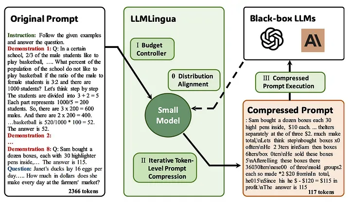
图 4：LLMLingua 方法的架构概览。来源：LLMLingua[2]

与 Selective Context 相比，LLMLingua 能更有效地保留提示词中的关键信息，同时还能够考虑到 tokens 之间的条件依赖关系，其压缩倍数可达 20 倍。

2.2 Budget controller

Budget controller 是 LLMLingua 的关键组件，用于为原始提示词的不同部分动态分配不同的压缩率。

考虑到提示词各部分对压缩行为的敏感程度各不相同 ------ 例如，问题需要保持较高的信息密度，而演示样例部分则可适度压缩。budget controller 的职责就在于此：对指导性提示词和问题采用较低的压缩比率，确保核心信息的完整留存；而对于演示样例部分，则可实施更高比率的压缩，剔除不必要的冗余信息。

budget controller 的具体算法，详述于图 5 中。

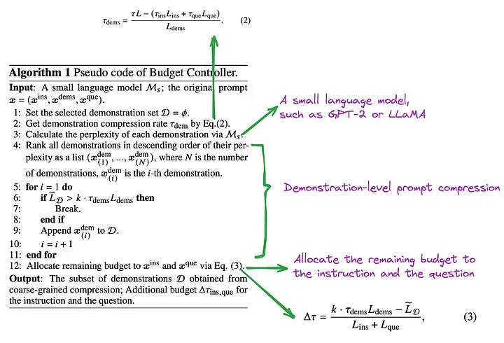
图 5：budget controller 的具体算法。Source: LLMLingua[2]

其核心变量定义如下：

Mₛ: 小型语言模型，比如 GPT-2 或 LLaMA。
x = (x^ins , x^dems , x^que) : 原始提示词，整合了指导性提示词、演示样例与问题三大部分。
L, L_ins, L_dems, 和 L_que 分别代表 x, x^ins , x^dems, 和 x^que 中的 token 总数。
𝜏_dems: 在总体压缩率 τ 的约束下，依据指导性提示词和问题预设的压缩率 τ_ins 和 τ_que 来决定的演示样例压缩率。
D: 集合 D 将收纳所有经过压缩处理后的演示样例。

主要操作步骤如下：

确定演示样例的压缩比例。
利用小型语言模型（如 GPT-2 或 LLaMA）计算原始演示样例集合中每个演示样例的困惑度（perplexity）。
按照困惑度从高到低排序全部演示样例。
迭代挑选演示样例并将其添加到集合 D。
完成演示样例的压缩后，将未使用的 budget （译者注：在总体压缩率的限制下，算法会优先确保演示样例被充分压缩，然后利用剩下的压缩能力去进一步压缩指导性提示词和问题，以实现最佳的信息保留和资源利用平衡。）转用于指导性提示词和问题的处理。
输出经过粗粒度压缩后的集合 D。

借助 demonstration-level （译者注：在完整的演示案例上进行压缩或处理，而不是单独处理每个小的组成部分（比如单词或短语）。）的压缩流程，budget controller 可以确保在削减数据量的同时，核心信息得以保全，能够有效实现原始提示词的瘦身。这一策略特别适合处理包含多重演示样例的复杂提示词。

涉及的程序代码，可在 control_context_budget 函数[14]中找到实现细节。

2.3 Iterative Token-level Prompt Compression (ITPC)

利用困惑度（perplexity）作为压缩标准，有其内在的局限性：the independence assumption（译者注：假设文本序列中的每个词汇（token）或字符的出现是彼此独立的，其出现的概率只依赖于它前面的一个或几个词汇，而与序列中更远的其他词汇无关。）。该假设认为每个 token 在提示词中孤立存在，其出现的概率仅取决于紧邻的前一个token，而不受其他任何 tokens 的影响。

然而，这一假设忽略了自然语言中词元（token）间错综复杂的相互依存关系，而这种关系对于理解上下文和保持语义的完整性至关重要。

忽略这些相互依存的关系，极有可能在压缩过程中造成重要信息的流失。 例如，在进行高比例压缩时，倘若某个 token 承载着上下文中的核心推理环节或逻辑联系纽带，那么仅仅依据其困惑度判定其去留，可能会导致推理链的断裂。

为克服这一挑战，LLMLingua 引入了 Iterative Token-level Prompt Compression（ITPC）算法。不同于仅凭独立概率评判 token 价值的传统方法，ITPC 算法在压缩提示词时，会更精细地评估每个 token 的实际贡献。通过反复审视提示词的每一部分，同时考量当前上下文中每个 token 的条件概率，这一算法能更有效地维系 token 间的内在联系，确保压缩后提示词的语义完整性和逻辑连贯性。

图 6 展示了 ITPC 算法的详细步骤：

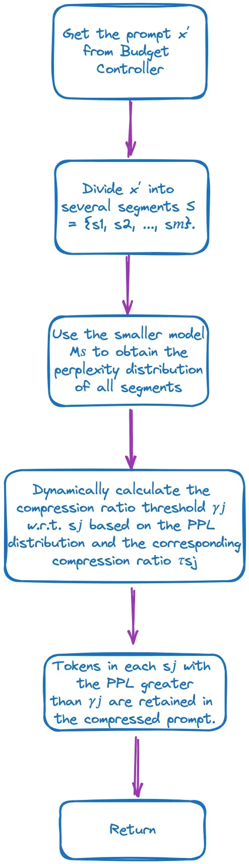
图 6：ITPC 算法的详细步骤。图片由原文作者提供

借助这一流程，ITPC 算法可以有效缩短提示词信息的长度，同时还能确保其语义内容的完整性，进而有效地降低了 LLM 的推理成本。

相关的实现代码可以在函数 iterative_compress_prompt[15] 中找到。

2.4 Instruction Tuning 指令调优

如图 4 所示，在 LLMLingua 框架内，指令调优（instruction tuning）扮演着至关重要的角色。该步骤的核心目的是缩小用于提示词压缩的小型语言模型与大语言模型(LLMs)之间在分布特性上的差异。

图 7 展示了 Instruction Tuning 算法的详细步骤：

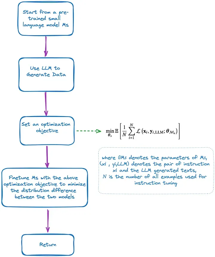
图 7：Instruction Tuning 的详细步骤。图片由原文作者提供

2.5 Code Demonstration 代码演示

我们现在开始展示代码。首要步骤是配置好环境。

(base) Florian:~ Florian$ conda create -n "llmlingua" python=3.11

(base) Florian:~ Florian$ conda activate llmlingua

(llmlingua) Florian:~ Florian$ pip install llmlingua

以下是已安装的版本信息：

llmlingua          0.2.1

下面是用于测试的代码段：

from llmlingua import PromptCompressor

GSM8K_PROMPT = "Question: Angelo and Melanie want to plan how many hours over the next week they should study together for their test next week. They have 2 chapters of their textbook to study and 4 worksheets to memorize. They figure out that they should dedicate 3 hours to each chapter of their textbook and 1.5 hours for each worksheet. If they plan to study no more than 4 hours each day, how many days should they plan to study total over the next week if they take a 10-minute break every hour, include 3 10-minute snack breaks each day, and 30 minutes for lunch each day?\nLet's think step by step\nAngelo and Melanie think they should dedicate 3 hours to each of the 2 chapters, 3 hours x 2 chapters = 6 hours total.\nFor the worksheets they plan to dedicate 1.5 hours for each worksheet, 1.5 hours x 4 worksheets = 6 hours total.\nAngelo and Melanie need to start with planning 12 hours to study, at 4 hours a day, 12 / 4 = 3 days.\nHowever, they need to include time for breaks and lunch. Every hour they want to include a 10-minute break, so 12 total hours x 10 minutes = 120 extra minutes for breaks.\nThey also want to include 3 10-minute snack breaks, 3 x 10 minutes = 30 minutes.\nAnd they want to include 30 minutes for lunch each day, so 120 minutes for breaks + 30 minutes for snack breaks + 30 minutes for lunch = 180 minutes, or 180 / 60 minutes per hour = 3 extra hours.\nSo Angelo and Melanie want to plan 12 hours to study + 3 hours of breaks = 15 hours total.\nThey want to study no more than 4 hours each day, 15 hours / 4 hours each day = 3.75\nThey will need to plan to study 4 days to allow for all the time they need.\nThe answer is 4\n\nQuestion: You can buy 4 apples or 1 watermelon for the same price. You bought 36 fruits evenly split between oranges, apples and watermelons, and the price of 1 orange is $0.50. How much does 1 apple cost if your total bill was $66?\nLet's think step by step\nIf 36 fruits were evenly split between 3 types of fruits, then I bought 36/3 = 12 units of each fruit\nIf 1 orange costs $0.50 then 12 oranges will cost $0.50 * 12 = $6\nIf my total bill was $66 and I spent $6 on oranges then I spent $66 - $6 = $60 on the other 2 fruit types.\nAssuming the price of watermelon is W, and knowing that you can buy 4 apples for the same price and that the price of one apple is A, then 1W=4A\nIf we know we bought 12 watermelons and 12 apples for $60, then we know that $60 = 12W + 12A\nKnowing that 1W=4A, then we can convert the above to $60 = 12(4A) + 12A\n$60 = 48A + 12A\n$60 = 60A\nThen we know the price of one apple (A) is $60/60= $1\nThe answer is 1\n\nQuestion: Susy goes to a large school with 800 students, while Sarah goes to a smaller school with only 300 students.  At the start of the school year, Susy had 100 social media followers.  She gained 40 new followers in the first week of the school year, half that in the second week, and half of that in the third week.  Sarah only had 50 social media followers at the start of the year, but she gained 90 new followers the first week, a third of that in the second week, and a third of that in the third week.  After three weeks, how many social media followers did the girl with the most total followers have?\nLet's think step by step\nAfter one week, Susy has 100+40 = 140 followers.\nIn the second week, Susy gains 40/2 = 20 new followers.\nIn the third week, Susy gains 20/2 = 10 new followers.\nIn total, Susy finishes the three weeks with 140+20+10 = 170 total followers.\nAfter one week, Sarah has 50+90 = 140 followers.\nAfter the second week, Sarah gains 90/3 = 30 followers.\nAfter the third week, Sarah gains 30/3 = 10 followers.\nSo, Sarah finishes the three weeks with 140+30+10 = 180 total followers.\nThus, Sarah is the girl with the most total followers with a total of 180.\nThe answer is 180"

llm_lingua = PromptCompressor()

## Or use the phi-2 model,
# llm_lingua = PromptCompressor("microsoft/phi-2")

## Or use the quantation model, like TheBloke/Llama-2-7b-Chat-GPTQ, only need <8GB GPU memory.
## Before that, you need to pip install optimum auto-gptq
# llm_lingua = PromptCompressor("TheBloke/Llama-2-7b-Chat-GPTQ", model_config={"revision": "main"})

compressed_prompt = llm_lingua.compress_prompt(GSM8K_PROMPT.split("\n\n")[0], instruction="", question="", target_token=200)

print('-' * 100)
print("original:")
print(GSM8K_PROMPT.split("\n\n")[0])

print('-' * 100)
print("compressed_prompt:")
print(compressed_prompt)

首次运行时会自动下载默认模型。当然，我们也有另一个选项，即使用量化模型（quantized model）。相关的运行结果展示在图 8 中：

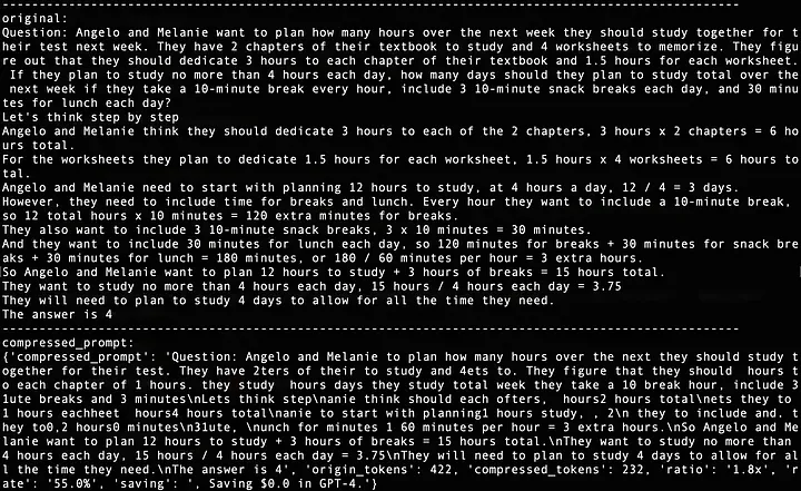
图 8 ：LLMLingua 测试代码的运行结果。此截图由原文作者提供

03 LongLLMLingua

LLMLingua 的问题在于，在压缩处理过程中忽略了用户提出的问题，这可能导致一些无关紧要的信息被无谓地保留下来。

而 LongLLMLingua[3] 的设计初衷正是为了解决这一缺陷，它创新性地在压缩流程中融入了对用户问题的考量和处理。

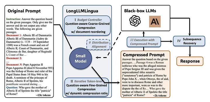
图 9：LongLLMLingua 框架，灰色斜体内容与 LLMLingua 相同。图片来源：LongLLMLingua[3]

如图 9 所示，LongLLMLingua 框架引入了四项新功能，以提升大语言模型识别关键信息的能力：

针对用户问题的粗粒度和细粒度两级压缩技术（Question-aware coarse-grained and fine-grained compression）；
动态调整的文档排序机制（Document reordering mechanism）；
可变的压缩比例设定（Dynamic compression ratio）；
子序列恢复算法（Subsequence recovery algorithm）。

3.1 针对用户问题的粗粒度压缩技术

LongLLMLingua 推荐采用这样一种方法，利用在不同文档上下文 x^doc_k 背景下问题 x^que 的困惑度，来衡量两者间的关联强度。我们可以在问题 x^que 后面附加一句限定语 x^restrict = "我们可以在提供的文档里找到这个问题的答案"。这样做的目的是强化 x^que 与 x^doc_k 之间的联系，同时，这句话作为一个正则化项（regularization item），能有效降低模型产生不切实际的预测结果的可能性。这可以表示为：

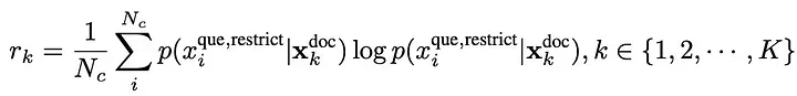
为什么不直接计算在问题 x^que 约束下的整体文档困惑度呢？原因在于，文档内往往充斥着许多与问题不相关的冗余信息。即便是在 x^que 的引导下，对整篇文档计算出的困惑度值也可能不够明显，从而导致它无法成为评估文档层面压缩效果的理想指标。

可以在函数 get_distance_longllmlingua[16] 中找到实现这一技术的相关代码。

3.2 针对用户问题的细粒度压缩技术

LongLLMLingua 引入了对比困惑度（contrastive perplexity）的概念。

首先，我们计算一个 token 的困惑度，不考虑问题的情况下，表示为 perplexity(x_i | x<i) 。然后，我们再次测量困惑度，这次包括了问题，表示为 perplexity(x_i | x^que, x<i)。这衡量的是在给定问题 x^que 的情况下，词元 x_i 对之前所有词元（token）的惊讶程度。

我们的目标是确定每个 token 的惊讶程度随问题变化的程度。如果当问题被包括进来后，某个词变得不那么令人惊讶，那么这个词很可能与问题高度相关。

3.3 动态调整的文档排序机制

如图 10 所示，在推理阶段，大语言模型(LLMs)倾向于利用提示词信息的起始和尾部内容，而往往忽视了其中间部分的信息，这便是所谓的"Lost in the Middle"问题。

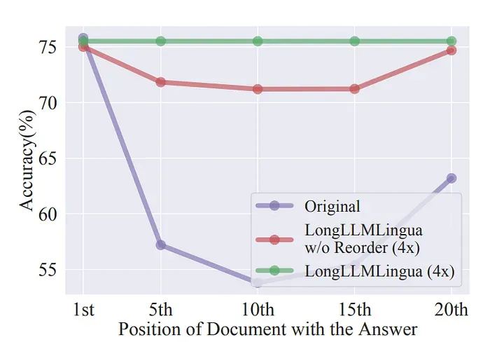
图 10：大语言模型(LLM)对相关资讯的把握能力受到其在提示词信息中位置的影响。为了解决中间信息丢失的问题，我们引入了一项文档重排序机制。图片来源：LongLLMLingua[3]

图 10 进一步表明，当关键信息被置于开头时，LLMs 的表现最为出色。基于此， LongLLMLingua 会根据粗粒度压缩的结果来组织段落，从前往后依据评分高低进行排序。

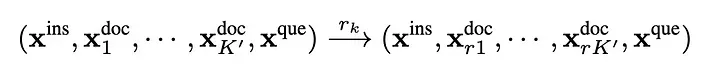
3.4 可变的压缩比例设定

鉴于不同文档中关键信息的密集程度存在差异，我们应当对那些与问题更加相关的文档分配更多资源（即采取更低的压缩比率）。

LongLLMLingua 运用在粗粒度压缩过程中得出的重要性得分，来指引细粒度压缩阶段的资源分配策略。

具体操作如下：首先，通过 LLMLingua 的 budget controller 为保留的文档设定初始资源量。随后，在细粒度压缩阶段，为每个文档动态分配资源。这一分配策略基于文档在粗粒度压缩阶段确定的重要性得分排名，以排名顺序作为资源分配依据。

LongLLMLingua 实施了一种线性调度方法（linear scheduler），实现资源的自适应分配（adaptive allocation）。对于每个词元（token） xi，其资源量计算公式如下：

其中，Nd表示所有文档的数量，𝛿𝜏是一个控制动态分配总资源量的超参数。

对应的源代码可以在 get_dynamic_compression_ratio[17] 函数中找到。

3.5 子序列恢复算法

如图 11 所示，在细粒度的逐 token 压缩环节中，一些关键实体的 token 有被丢弃的风险。例如，"2009"在原始提示词中可能被压缩至"209"，"Wilhelm Conrad Rontgen"也可能被简化压缩为"Wilhelmgen"。

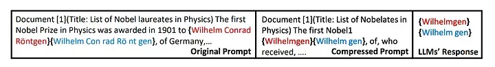
图 11：展示了一个子序列恢复算法案例，其中红色文本代表原始内容，而蓝色文字则是经过压缩后的结果。来源：LongLLMLingua[3]

LongLLMLingua 设计了一套子序列恢复算法，能够从大语言模型(LLMs)的回应中复原原始信息，如图 12 所示。

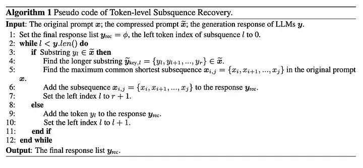
图 12：子序列恢复算法流程图。图片来源：LongLLMLingua

其核心流程包括以下几个步骤：

遍历大语言模型(LLM)响应内容中的每一个词元（token）yl，从中选取在压缩提示词 x˜ 中出现的最长子序列 y˜key,l；
在原始提示词 x 内，寻找与 y˜key,l 匹配的最大公共最短子序列（maximum common shortest subsequence）xi,j；
将大语言模型(LLMs)响应内容中的相应词元 y˜key,l 替换为原始的 xi,j。

这一算法的具体代码可以在 recover 函数[18]中找到。

3.6 代码演示

环境配置的方法与 LLMLingua 相同。下面是测试代码：

from llmlingua import PromptCompressor

GSM8K_PROMPT = "Question: Angelo and Melanie want to plan how many hours over the next week they should study together for their test next week. They have 2 chapters of their textbook to study and 4 worksheets to memorize. They figure out that they should dedicate 3 hours to each chapter of their textbook and 1.5 hours for each worksheet. If they plan to study no more than 4 hours each day, how many days should they plan to study total over the next week if they take a 10-minute break every hour, include 3 10-minute snack breaks each day, and 30 minutes for lunch each day?\nLet's think step by step\nAngelo and Melanie think they should dedicate 3 hours to each of the 2 chapters, 3 hours x 2 chapters = 6 hours total.\nFor the worksheets they plan to dedicate 1.5 hours for each worksheet, 1.5 hours x 4 worksheets = 6 hours total.\nAngelo and Melanie need to start with planning 12 hours to study, at 4 hours a day, 12 / 4 = 3 days.\nHowever, they need to include time for breaks and lunch. Every hour they want to include a 10-minute break, so 12 total hours x 10 minutes = 120 extra minutes for breaks.\nThey also want to include 3 10-minute snack breaks, 3 x 10 minutes = 30 minutes.\nAnd they want to include 30 minutes for lunch each day, so 120 minutes for breaks + 30 minutes for snack breaks + 30 minutes for lunch = 180 minutes, or 180 / 60 minutes per hour = 3 extra hours.\nSo Angelo and Melanie want to plan 12 hours to study + 3 hours of breaks = 15 hours total.\nThey want to study no more than 4 hours each day, 15 hours / 4 hours each day = 3.75\nThey will need to plan to study 4 days to allow for all the time they need.\nThe answer is 4\n\nQuestion: You can buy 4 apples or 1 watermelon for the same price. You bought 36 fruits evenly split between oranges, apples and watermelons, and the price of 1 orange is $0.50. How much does 1 apple cost if your total bill was $66?\nLet's think step by step\nIf 36 fruits were evenly split between 3 types of fruits, then I bought 36/3 = 12 units of each fruit\nIf 1 orange costs $0.50 then 12 oranges will cost $0.50 * 12 = $6\nIf my total bill was $66 and I spent $6 on oranges then I spent $66 - $6 = $60 on the other 2 fruit types.\nAssuming the price of watermelon is W, and knowing that you can buy 4 apples for the same price and that the price of one apple is A, then 1W=4A\nIf we know we bought 12 watermelons and 12 apples for $60, then we know that $60 = 12W + 12A\nKnowing that 1W=4A, then we can convert the above to $60 = 12(4A) + 12A\n$60 = 48A + 12A\n$60 = 60A\nThen we know the price of one apple (A) is $60/60= $1\nThe answer is 1\n\nQuestion: Susy goes to a large school with 800 students, while Sarah goes to a smaller school with only 300 students.  At the start of the school year, Susy had 100 social media followers.  She gained 40 new followers in the first week of the school year, half that in the second week, and half of that in the third week.  Sarah only had 50 social media followers at the start of the year, but she gained 90 new followers the first week, a third of that in the second week, and a third of that in the third week.  After three weeks, how many social media followers did the girl with the most total followers have?\nLet's think step by step\nAfter one week, Susy has 100+40 = 140 followers.\nIn the second week, Susy gains 40/2 = 20 new followers.\nIn the third week, Susy gains 20/2 = 10 new followers.\nIn total, Susy finishes the three weeks with 140+20+10 = 170 total followers.\nAfter one week, Sarah has 50+90 = 140 followers.\nAfter the second week, Sarah gains 90/3 = 30 followers.\nAfter the third week, Sarah gains 30/3 = 10 followers.\nSo, Sarah finishes the three weeks with 140+30+10 = 180 total followers.\nThus, Sarah is the girl with the most total followers with a total of 180.\nThe answer is 180"
QUESTION = "Question: Josh decides to try flipping a house.  He buys a house for $80,000 and then puts in $50,000 in repairs.  This increased the value of the house by 150%.  How much profit did he make?"



llm_lingua = PromptCompressor()

compressed_prompt = llm_lingua.compress_prompt(
    GSM8K_PROMPT.split("\n\n")[0],
    question = QUESTION,
 # ratio=0.55
 # Set the special parameter for LongLLMLingua
    condition_in_question = "after_condition",
    reorder_context = "sort",
    dynamic_context_compression_ratio = 0.3, # or 0.4
    condition_compare = True,
    context_budget = "+100",
    rank_method = "longllmlingua",
)

print('-' * 100)
print("original:")
print(GSM8K_PROMPT.split("\n\n")[0])


print('-' * 100)
print("compressed_prompt:")
print(compressed_prompt)

运行结果如图 13 所示：

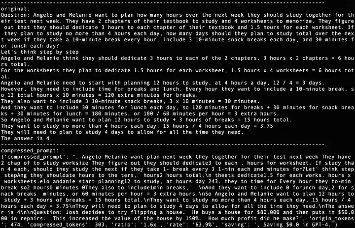
图 13：LongLLMLingua 测试代码的运行结果。截图由作者提供。

04 AutoCompressor

不同于先前提及的方法，AutoCompressor[4] 采取了一种基于软提示词的创新途径。

它巧妙地通过增加词汇量和利用"summary tokens"和"summary vectors"来提炼大量上下文信息，进而精调现有的模型结构。

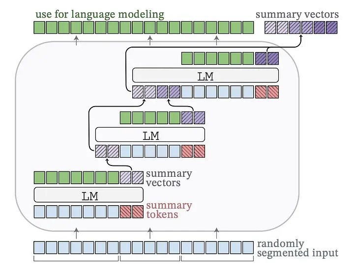
图 14：AutoCompressor 通过递归生成 summary vectors 来处理长文档，这些 summary vectors 作为软提示词（soft prompts）被传递给后续的所有文档片段。图片来源：AutoCompressor[4]

图 14 描绘了 AutoCompressor 的工作原理，其运行步骤如下：

词汇扩展（Expand Vocabulary） ：在这一步骤中，我们将 “summary tokens” 加入到模型现有的词汇库中。这些 tokens 的作用是帮助模型将庞大的信息量压缩成更紧凑的向量表征。
文档分割（Split Document） ：待处理的文档被切割成若干小段，每一小段后都会附加有 summary tokens 。这些 tokens 不仅携带了本段的信息，还包含了前面所有段落的摘要信息，实现了摘要信息的连续积累（summary accumulation）。
微调训练（Fine-tuning Training） ：采用无监督训练的方式，借助 “next word prediction” 任务对模型进行微调。该任务的核心在于，根据当前片段前的 tokens 序列以及之前片段的摘要向量（summary vectors），预测下一个单词。
反向传播（Backpropagation） ：AutoCompressor 在每个文档片段上运用 backpropagation through time(BPTT)（译者注：对于每一个时间步，BPTT 都会计算损失函数关于当前时间步和所有之前时间步参数的梯度，然后将这些梯度反向传播回网络，以更新参数。）和 gradient checkpointing（译者注：在标准的反向传播过程中，为了计算梯度，需要保存前向传播过程中的所有中间结果。但随着网络深度的增加，这会消耗大量的内存。Gradient checkpointing 通过牺牲一些计算效率来减少内存需求。）技术，能够有效缩减计算图（computational graph）的规模。反向传播针对整个文档进行，使得模型能够全面理解并学习到整个上下文之间存在的关联。

4.1 代码演示

AutoCompressor[19] 开放了其源代码，感兴趣的读者可以试着读一读。

import torch
from transformers import AutoTokenizer
from auto_compressor import LlamaAutoCompressorModel, AutoCompressorModel

# Load AutoCompressor trained by compressing 6k tokens in 4 compression steps
tokenizer = AutoTokenizer.from_pretrained("princeton-nlp/AutoCompressor-Llama-2-7b-6k")
# Need bfloat16 + cuda to run Llama model with flash attention
model = LlamaAutoCompressorModel.from_pretrained("princeton-nlp/AutoCompressor-Llama-2-7b-6k", torch_dtype=torch.bfloat16).eval().cuda()

prompt = 'The first name of the current US president is "'
prompt_tokens = tokenizer(prompt, add_special_tokens=False, return_tensors="pt").input_ids.cuda()

context = """Joe Biden, born in Scranton, Pennsylvania, on November 20, 1942, had a modest upbringing in a middle-class family. He attended the University of Delaware, where he double-majored in history and political science, graduating in 1965. Afterward, he earned his law degree from Syracuse University College of Law in 1968.\nBiden's early political career began in 1970 when he was elected to the New Castle County Council in Delaware. In 1972, tragedy struck when his wife Neilia and 1-year-old daughter Naomi were killed in a car accident, and his two sons, Beau and Hunter, were injured. Despite this devastating loss, Biden chose to honor his commitment and was sworn in as a senator by his sons' hospital bedsides.\nHe went on to serve as the United States Senator from Delaware for six terms, from 1973 to 2009. During his time in the Senate, Biden was involved in various committees and was particularly known for his expertise in foreign affairs, serving as the chairman of the Senate Foreign Relations Committee on multiple occasions.\nIn 2008, Joe Biden was selected as the running mate for Barack Obama, who went on to win the presidential election. As Vice President, Biden played an integral role in the Obama administration, helping to shape policies and handling issues such as economic recovery, foreign relations, and the implementation of the Affordable Care Act (ACA), commonly known as Obamacare.\nAfter completing two terms as Vice President, Joe Biden decided to run for the presidency in 2020. He secured the Democratic nomination and faced the incumbent President Donald Trump in the general election. Biden campaigned on a platform of unity, promising to heal the divisions in the country and tackle pressing issues, including the COVID-19 pandemic, climate change, racial justice, and economic inequality.\nIn the November 2020 election, Biden emerged victorious, and on January 20, 2021, he was inaugurated as the 46th President of the United States. At the age of 78, Biden became the oldest person to assume the presidency in American history.\nAs President, Joe Biden has worked to implement his agenda, focusing on various initiatives, such as infrastructure investment, climate action, immigration reform, and expanding access to healthcare. He has emphasized the importance of diplomacy in international relations and has sought to rebuild alliances with global partners.\nThroughout his long career in public service, Joe Biden has been recognized for his commitment to bipartisanship, empathy, and his dedication to working-class issues. He continues to navigate the challenges facing the nation, striving to bring the country together and create positive change for all Americans."""
context_tokens = tokenizer(context, add_special_tokens=False, return_tensors="pt").input_ids.cuda()

summary_vectors = model(context_tokens, output_softprompt=True).softprompt
print(f"Compressing {context_tokens.size(1)} tokens to {summary_vectors.size(1)} summary vectors")
# >>> Compressing 660 tokens to 50 summary vectors

generation_with_summary_vecs = model.generate(prompt_tokens, do_sample=False, softprompt=summary_vectors, max_new_tokens=12)[0]
print("Generation w/ summary vectors:\n" + tokenizer.decode(generation_with_summary_vecs))
# >>> The first name of the current US president is "Joe" and the last name is "Biden".

next_tokens_without_context = model.generate(prompt_tokens, do_sample=False, max_new_tokens=11)[0]
print("Generation w/o context:\n" + tokenizer.decode(next_tokens_without_context))
# >>> The first name of the current US president is "Donald" and the last name is "Trump".

05 LLMLingua-2

LLMLingua-2[6] 发现，通过基于因果语言模型（如LLaMa-7B）的信息熵删除 tokens 或词汇单位（lexical units）来进行提示词压缩存在两大挑战：

(1) 用来计算信息熵的小型语言模型与提示词压缩的实际目标不一致。

(2) 这一方法仅依赖于单向的上下文信息，而这或许无法覆盖提示词压缩所需的所有必要信息。

这些问题的核心在于，基于信息熵（information entropy）进行提示词压缩可能并非是最优的选择。

LLMLingua-2 的整体架构如图 15 所示：

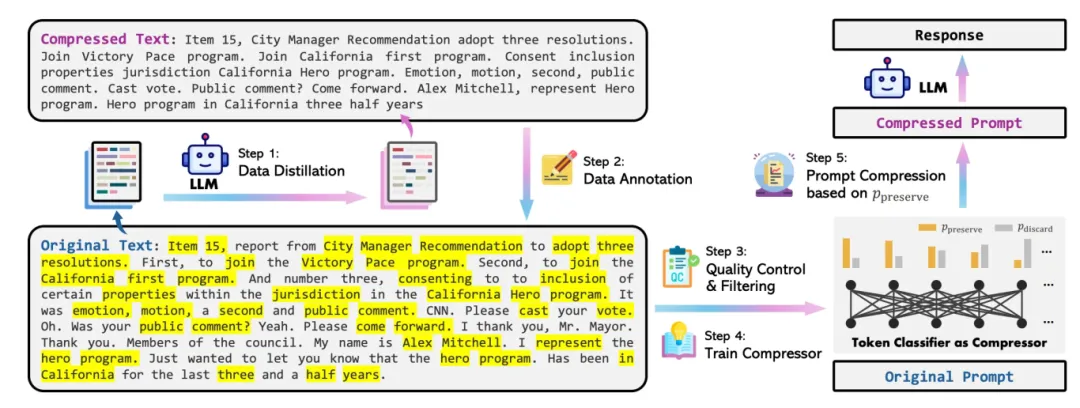
图 15：LLMLingua-2的架构总览。来源：LLMLingua-2[6]

针对第一个问题，LLMLingua-2 引入了数据蒸馏流程。该流程从大语言模型中提取知识，在不丢失关键信息的情况下压缩提示词。同时，它还构建了一个 extractive text compression dataset （译者注：从原始文本中挑选出最重要的句子、短语或词汇，直接组成一个较短的版本，以保留原文的主要信息和意义。一般来说不涉及生成新的句子来概括原文）。在这样的数据集上进行训练，有助于小型语言模型更精准地对齐提示词压缩的需求。

面对第二个问题，LLMLingua-2 采取了一种创新策略 ------ 将提示词压缩转化为词元（token）分类任务。这一策略确保了压缩后的提示词能忠实地反映原始提示词的意图。它选用 transformer 的编码器作为底层架构，能够充分利用完整的双向上下文信息（bidirectional context），捕捉到进行提示词压缩所需的全部必要细节。

5.1 如何构建有效的提示词压缩数据集？

数据蒸馏

数据蒸馏从大语言模型（比如 GPT-4）中抽取知识，以便在不丢失基本信息的情况下实现有效压缩提示词。

在 LLMLingua-2 这一项目中，指导性提示词的设计经过了精心设计，如图 16 所示。这些指导性提示词（instructions）指导 GPT-4 在不向生成文本中引入新词汇的前提下，剔除原始文本中的冗余词汇，从而实现文本的压缩。

与此同时，这些指导性提示词（instructions）并未强行规定压缩的比例。相反，GPT-4 被鼓励尽可能地缩减原始文本的体积，但前提是必须确保原始信息的完整性。

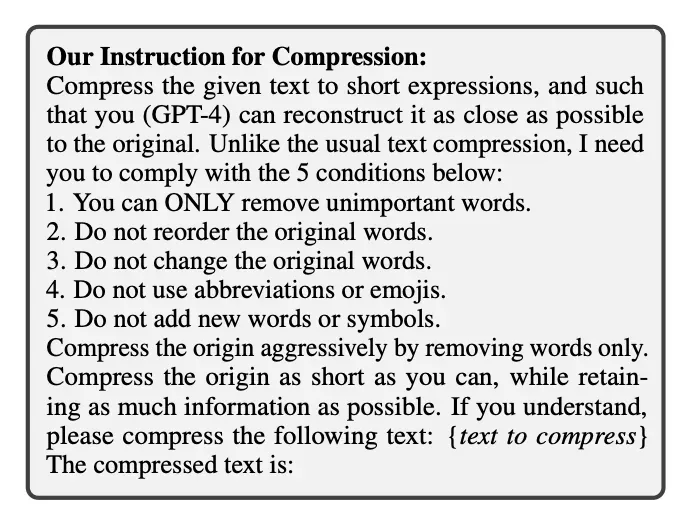
图 16：LLMLingua-2 中用于数据蒸馏的指导性提示词。

如图 17 所示，在处理非常长的文本时，GPT-4 倾向于采取高比例的压缩策略。可能是因为其处理长文本的能力有限。这种激进的压缩策略往往伴随着大量信息的流失，可能严重影响接下来的任务执行效果。

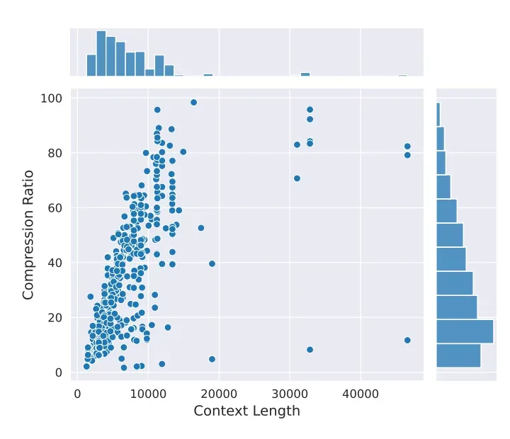
图 17：在 MeetingBank 数据集上，根据原始文本长度，GPT-4 的压缩比情况。在本研究中，我们使用了 GPT-4–32k ，并将输出 tokens 的数量上限设为 4096。来源：LLMLingua-2[6]。

为了解决这个问题，LLMLingua-2 引入了一种分块压缩（chunk compression） 技术，即先将长文本拆解为若干个不超过 512 tokens 的小文本块，再分别对每一小文本块进行压缩处理，由 GPT-4 来完成这一过程。

数据标注

现在，我们已经利用数据蒸馏手段，收集到了原始文本与其压缩内容的组合。数据标注的目的是为原始文本里的每个 token 标上一个二元标签，以此判断压缩后该字符是否应该被保留。

考虑到 GPT-4 不一定能够完美遵循指导性提示词，LLMLingua-2 采取了滑动窗口策略（sliding window） ，以此来限定搜索范围。同时，还引入了模糊匹配技术（fuzzy matching） ，有效处理了 GPT-4 在提示词压缩过程中对原始词汇可能做出的细微改动。

质量控制

在 LLMLingua-2 项目中，质量控制环节采用了两个关键指标来评估通过 GPT-4 蒸馏生成的压缩文本，以及自动标注标签的优劣：Variation Rate（VR） 和Alignment Gap（AG） 。

Variation Rate（VR）衡量的是，压缩后的文本与原始文本相比，有多少比例的词汇发生了改变。而Alignment Gap（AG），则是用来衡量自动标注的标签的精准程度。

通过这些评估指标，LLMLingua-2 便能有效地筛除不合格的样本，从而保障整个数据集质量。

5.2 Compressor 压缩器

将其视为二元分类问题

从本质上讲，可将提示词压缩问题重塑为二元分类问题。其基本概念是将每一个词汇单元视为一个独立的实体，并为其分配一个标签："保留" 或 "丢弃"。这一策略不仅确保了压缩后提示词内容的完整性，同时还简化了模型结构。

模型架构设计

采用了基于 Transformer 编码器的特征编码器（feature encoder），并在其上巧妙地叠加了一个线性分类层（linear classification layer）。

这样的架构设计使得模型能够深刻理解每个词汇单元的双向上下文信息，为高效完成压缩任务奠定了坚实的基础。

提示词压缩策略

压缩原始提示词 x 的策略分为三个步骤。目标压缩比率设定为 1/τ，这里 τ 即为压缩后提示词的词汇量与原始提示词 x 的词汇量之商。

首先，我们计算出压缩后提示词 x˜ 需要保留的 token 数量：N˜ = τN。
随后，运用 token 分类模型来预估每个词汇 xi 被标定为"保留"的概率 pi。
最后，我们从原始提示词 x 中筛选出前 N˜ 个 pi 值最高的词汇，严格保持其原有排列顺序，进而组成压缩后的提示词 x˜。

5.3 代码演示

从上文可以看出，LLMLingua-2 的主要工作是构建压缩器（compressor）。那么，当我们成功获取了这个压缩器之后，下一步该如何操作呢？

请参照下方的代码示例（环境配置方式与 LLMLingua 一致）。compress_prompt_llmlingua2[20] 函数内集中体现了主要的处理逻辑。

from llmlingua import PromptCompressor

PROMPT = "John: So, um, I've been thinking about the project, you know, and I believe we need to, uh, make some changes. I mean, we want the project to succeed, right? So, like, I think we should consider maybe revising the timeline.\n\nSarah: I totally agree, John. I mean, we have to be realistic, you know. The timeline is, like, too tight. You know what I mean? We should definitely extend it."

llm_lingua = PromptCompressor(
    model_name = "microsoft/llmlingua-2-xlm-roberta-large-meetingbank",
    use_llmlingua2 = True,
)
compressed_prompt = llm_lingua.compress_prompt(PROMPT, rate=0.33, force_tokens = ['\n', '?'])

## Or use LLMLingua-2-small model
# llm_lingua = PromptCompressor(
#     model_name="microsoft/llmlingua-2-bert-base-multilingual-cased-meetingbank",
#     use_llmlingua2=True,
# )

print('-' * 100)
print("original:")
print(PROMPT)

print('-' * 100)
print("compressed_prompt:")
print(compressed_prompt)

运行结果如图 18 所示：

图 18：LLMLingua-2 测试代码的运行结果。截图由原文作者提供

06 RECOMP

RECOMP[7] 创新性地引入了两类经过训练的压缩器：抽取型（extractive）和概括型（abstractive）。抽取型压缩器擅长从已检索的文档中精挑细选出有价值的部分 ；而概括型压缩器则通过融合多篇文档的精华，自动生成摘要。

图 19 生动描绘了压缩器在 RECOMP 架构中的位置。

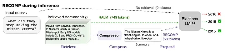
图 19：RECOMP 架构。图片来源：RECOMP

6.1 抽取型压缩器

给定输入文档集中的 n 个句子 [s1, s2, ..., sn] ，使用一个双编码器模型（dual encoder model）进行训练。该模型能将每个句子 si 和输入序列 x 转换为固定长度的向量表征。这些嵌入向量的内积反映了将句子 si 添加到输入序列 x 中，对于大语言模型（LLM）生成目标输出序列（target output sequence）的帮助程度。

压缩器最终生成的摘要 s 由排名前 N 的句子组成，按照它们与输入序列的内积进行排序。

6.2 概括型压缩器

概括型压缩器采用的是编码器-解码器架构（encoder-decoder）。它处理输入序列 x 与检索出的文档集合并将其连接起来，进而产生摘要 s。

该方法具体步骤如下：首先利用大语言模型（如GPT-3）来生成训练数据集；然后对数据集进行筛选；最后，使用经过筛选后的数据集来训练编码器-解码器模型（encoder-decoder model）。

6.3 代码演示

鉴于 RECOMP 当前尚处在开发初期，我们在此暂不进行演示。对此感兴趣的读者不妨亲自动手体验一番。

07 结论 Conclusion

本文探讨了提示词压缩技术，覆盖了该技术的方法分类、算法原理以及代码实践演示。

在本文所讨论的各种方法中，LongLLMLingua 或许是一个更为出色的选择 。我们已在项目实践中应用了这一方法。原文作者承诺一旦他们发现了 LongLLMLingua 存在的不足，或是发现了更为优秀的替代方案，他们将对原文（https://ai.gopubby.com/advanced-rag-09-prompt-compression-95a589f7b554 ）进行更新（译者注：如果有小伙伴关注到了内容更新，请在下方留言，我们会尽量及时进行内容补充，感谢❤️。）。此外，LLMLingua-2 也值得一试，它在运行速度和内存消耗方面都表现优异。

Thanks for reading!

Florian June

An artificial intelligence researcher, mainly write articles about Large Language Models, data structures and algorithms, and NLP.

END

参考资料

[1]https://arxiv.org/pdf/2304.12102.pdf

[2]https://arxiv.org/pdf/2310.05736.pdf

[3]https://arxiv.org/pdf/2310.06839.pdf

[4]https://arxiv.org/pdf/2305.14788.pdf

[5]https://arxiv.org/pdf/2304.08467.pdf

[6]https://arxiv.org/pdf/2403.12968.pdf

[7]https://arxiv.org/pdf/2310.04408.pdf