傅里叶级数与傅里叶变换
背景
傅里叶级数和傅里叶变换是数学和工程领域中的重要工具,特别是在信号处理、图像处理和物理学中。傅里叶级数用于将周期函数表示为正弦和余弦函数的和,而傅里叶变换用于将任意函数表示为频率的函数。
公式
-
傅里叶级数:给定周期函数 f ( t ) f(t) f(t),其傅里叶级数表示为:
f ( t ) = a 0 + ∑ n = 1 ∞ ( a n cos ( 2 π n t T ) + b n sin ( 2 π n t T ) ) f(t) = a_0 + \sum_{n=1}^{\infty} \left( a_n \cos \left( \frac{2\pi n t}{T} \right) + b_n \sin \left( \frac{2\pi n t}{T} \right) \right) f(t)=a0+n=1∑∞(ancos(T2πnt)+bnsin(T2πnt))
其中:
a 0 = 1 T ∫ 0 T f ( t ) d t a_0 = \frac{1}{T} \int_{0}^{T} f(t) \, dt a0=T1∫0Tf(t)dt
a n = 2 T ∫ 0 T f ( t ) cos ( 2 π n t T ) d t a_n = \frac{2}{T} \int_{0}^{T} f(t) \cos \left( \frac{2\pi n t}{T} \right) \, dt an=T2∫0Tf(t)cos(T2πnt)dt
b n = 2 T ∫ 0 T f ( t ) sin ( 2 π n t T ) d t b_n = \frac{2}{T} \int_{0}^{T} f(t) \sin \left( \frac{2\pi n t}{T} \right) \, dt bn=T2∫0Tf(t)sin(T2πnt)dt -
傅里叶变换:给定函数 f ( t ) f(t) f(t),其傅里叶变换表示为:
F ( f ) ( ω ) = F ( ω ) = ∫ − ∞ ∞ f ( t ) e − i ω t d t \mathcal{F}(f)(\omega) = F(\omega) = \int_{-\infty}^{\infty} f(t) e^{-i\omega t} \, dt F(f)(ω)=F(ω)=∫−∞∞f(t)e−iωtdt
其逆变换为:
f ( t ) = 1 2 π ∫ − ∞ ∞ F ( ω ) e i ω t d ω f(t) = \frac{1}{2\pi} \int_{-\infty}^{\infty} F(\omega) e^{i\omega t} \, d\omega f(t)=2π1∫−∞∞F(ω)eiωtdω
示例题目
题目:求周期函数 f ( t ) = t f(t) = t f(t)=t 在区间 [ − π , π ] [-\pi, \pi] [−π,π] 上的傅里叶级数表示。
详细讲解
- 计算
a
0
a_0
a0:
a 0 = 1 2 π ∫ − π π t d t = 0 a_0 = \frac{1}{2\pi} \int_{-\pi}^{\pi} t \, dt = 0 a0=2π1∫−ππtdt=0 - 计算
a
n
a_n
an:
a n = 1 π ∫ − π π t cos ( n t ) d t = 0 a_n = \frac{1}{\pi} \int_{-{\pi}}^{\pi} t \cos(nt) \, dt = 0 an=π1∫−ππtcos(nt)dt=0 - 计算
b
n
b_n
bn:
b n = 1 π ∫ − π π t sin ( n t ) d t = 2 ( − 1 ) n + 1 n b_n = \frac{1}{\pi} \int_{-\pi}^{\pi} t \sin(nt) \, dt = \frac{2(-1)^{n+1}}{n} bn=π1∫−ππtsin(nt)dt=n2(−1)n+1
因此,傅里叶级数为:
f
(
t
)
=
∑
n
=
1
∞
2
(
−
1
)
n
+
1
n
sin
(
n
t
)
f(t) = \sum_{n=1}^{\infty} \frac{2(-1)^{n+1}}{n} \sin(nt)
f(t)=n=1∑∞n2(−1)n+1sin(nt)
Python代码求解
import numpy as np
import matplotlib.pyplot as plt

# 定义周期函数
def f(t):
    return t

# 定义傅里叶级数展开的项数
N = 10

# 定义傅里叶级数
def fourier_series(t, N):
    result = np.zeros_like(t)
    for n in range(1, N + 1):
        result += (2 * (-1)**(n + 1) / n) * np.sin(n * t)
    return result

# 生成时间点
t = np.linspace(-np.pi, np.pi, 1000)

# 计算傅里叶级数近似
f_approx = fourier_series(t, N)

# 绘图
plt.plot(t, f(t), label='Original function')
plt.plot(t, f_approx, label='Fourier series approximation')
plt.legend()
plt.xlabel('t')
plt.ylabel('f(t)')
plt.title('Fourier Series Approximation')
plt.grid(True)
plt.show()
实际生活中的例子
在实际生活中,傅里叶变换用于信号处理,例如将音频信号转换为频谱,以分析不同频率的声音成分。傅里叶级数则在分析周期信号(如振动和电波)时非常有用。通过将复杂的周期信号分解为简单的正弦和余弦分量,可以更容易地理解和处理这些信号。
一个python例子
import numpy as np
import matplotlib.pyplot as plt
# 定义周期函数的频率和系数
T = 2 * np.pi # 周期
N = 5 # 傅里叶级数的项数
# 定义时间范围
t = np.linspace(-np.pi, np.pi, 1000)
# 定义傅里叶级数的各项
def fourier_series_terms(t, N):
terms = []
for n in range(1, N + 1):
term = (2 * (-1)**(n + 1) / n) * np.sin(n * t)
terms.append(term)
return terms
# 计算傅里叶级数的各项
terms = fourier_series_terms(t, N)
# 绘图
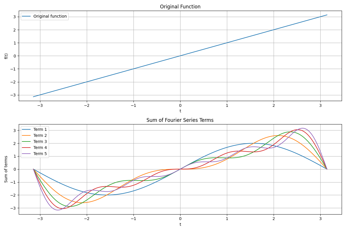
plt.figure(figsize=(12, 8))
# 原始函数
plt.subplot(2, 1, 1)
plt.plot(t, t, label='Original function')
plt.title('Original Function')
plt.xlabel('t')
plt.ylabel('f(t)')
plt.legend()
plt.grid(True)
# 各项的和
plt.subplot(2, 1, 2)
sum_terms = np.zeros_like(t)
for i, term in enumerate(terms):
sum_terms += term
plt.plot(t, sum_terms, label=f'Term {i+1}')
plt.title('Sum of Fourier Series Terms')
plt.xlabel('t')
plt.ylabel('Sum of terms')
plt.legend()
plt.grid(True)
plt.tight_layout()
plt.show()


![【2024最新华为OD-C/D卷试题汇总】[支持在线评测] 特惠寿司(100分) - 三语言AC题解(Python/Java/Cpp)](https://img-blog.csdnimg.cn/direct/47a1ce0444514757a0ccc2fb1f60306e.png)