opencv_特征检测和描述

理解特征

寻找独特的特定模式或特定特征，可以轻松跟踪和比较。

拼图：在图像中搜索这些特征，找到它们，在其他图像中查找相同的特征并对齐它们。而已。

基本上，角被认为是图像中的好特征。

在本单元中，我们正在寻找 OpenCV 中的不同算法来查找特征，描述特征，匹配它们等。

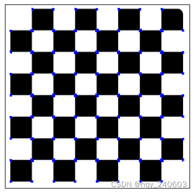
Harris 角点检测

OpenCV 中的 Harris 角点检测器

Harris角点检测的结果是一个由角点分数构成的灰度图像。选取适当的阈值对结果图像进行二值化我们就检测到了图像中的角点。

为此，OpenCV具有函数cv.cornerHarris()。它的参数是：

img - 输入图像，应该是灰度和float32类型。
blockSize - 考虑角点检测的邻域大小
ksize - 使用的Sobel衍生物的孔径参数。
k - 方程中的Harris检测器自由参数。

import numpy as np
import cv2 as cv
from matplotlib import pyplot as plt

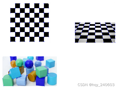
img1 = cv.imread('c:/Users/HP/Downloads/chessboard1.png')
img2 = cv.imread('c:/Users/HP/Downloads/chessboard2.png')
img3 = cv.imread('c:/Users/HP/Downloads/chessboard3.png')


gray = cv.cvtColor(img1,cv.COLOR_BGR2GRAY)
gray = np.float32(gray)
dst = cv.cornerHarris(gray,2,3,0.04)
#result is dilated for marking the corners, not important
dst = cv.dilate(dst,None)
# 阈值选择
img1[dst>0.01*dst.max()]=[0,0,255]

gray = cv.cvtColor(img2,cv.COLOR_BGR2GRAY)
gray = np.float32(gray)
dst = cv.cornerHarris(gray,2,3,0.04)
#result is dilated for marking the corners, not important
dst = cv.dilate(dst,None)
# 阈值选择
img2[dst>0.01*dst.max()]=[0,0,255]

gray = cv.cvtColor(img3,cv.COLOR_BGR2GRAY)
gray = np.float32(gray)
dst = cv.cornerHarris(gray,2,3,0.04)
#result is dilated for marking the corners, not important
dst = cv.dilate(dst,None)
# 阈值选择
img3[dst>0.01*dst.max()]=[0,0,255]


plt.figure()  

plt.subplot(2, 2, 1)  # (rows, columns, panel number)  
plt.imshow(img1)  
plt.axis('off')  # 关闭坐标轴  

plt.subplot(2, 2, 2)  # (rows, columns, panel number)  
plt.imshow(img2)  
plt.axis('off')  # 关闭坐标轴  

plt.subplot(2, 2, 3)  # (rows, columns, panel number)  
plt.imshow(img3)  
plt.axis('off')  # 关闭坐标轴  


plt.show()

在这里插入图片描述

具有亚像素级精度的角点

以最高精度找到角点：

OpenCV 带有一个函数 cv.cornerSubPix() ，它进一步细化了角点检测，以达到亚像素级精度：

先找到 Harris 角点，然后将这些角的质心（角点处可能有一堆像素，我们采用它们的质心）传递给该函数来细化它们；

在经过指定次数的迭代或达到一定精度后停止它，以先发生者为准。

Harris 角点以红色像素标记，细化后的角点以绿色像素标记。

import numpy as np
import cv2 as cv

img = img1
gray = cv.cvtColor(img,cv.COLOR_BGR2GRAY)

# find Harris corners
gray = np.float32(gray)
dst = cv.cornerHarris(gray,2,3,0.04)
dst = cv.dilate(dst,None)
ret, dst = cv.threshold(dst,0.01*dst.max(),255,0)
dst = np.uint8(dst)

# 找到质心
ret, labels, stats, centroids = cv.connectedComponentsWithStats(dst)

# 定义refine的标准
criteria = (cv.TERM_CRITERIA_EPS + cv.TERM_CRITERIA_MAX_ITER, 100, 0.001)
corners = cv.cornerSubPix(gray,np.float32(centroids),(5,5),(-1,-1),criteria)

# Now draw them
res = np.hstack((centroids,corners))
res = np.int0(res)
img[res[:,1],res[:,0]]=[0,0,255]
img[res[:,3],res[:,2]] = [0,255,0]

plt.xticks([]), plt.yticks([]) # 隐藏 X 和 Y 轴的刻度值
plt.imshow(img)

在这里插入图片描述

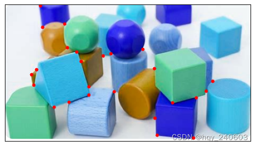
Shi-Tomasi 角点检测和追踪的良好特征

J. Shi 和 C. Tomasi 在他们的论文 Good Features to Track 中做了一个小修改，与 Harris 角点检测相比显示出更好的结果。

Harri 角点检测的评分由下式给出： $\lambda_1 \lambda_2 - k(\lambda_1+\lambda_2)^2$

不同于此，Shi-Tomasi 提出： $min(\lambda_1, \lambda_2)$

cv.goodFeaturesToTrack() 通过 Shi-Tomasi 方法（或 Harris 角点检测，如果你指定它）在图像中找到 N 个最佳的角点：

灰度图像；
指定要查找的角点数量；
然后指定质量等级，该等级是 0-1 之间的值，所有低于这个质量等级的角点都将被忽略；
最后设置检测到的两个角点之间的最小欧氏距离。

通过所有这些信息，该函数可以在图像中找到角点。所有低于质量等级的角点都将被忽略。然后它根据质量按降序对剩余的角点进行排序。该函数选定质量等级最高的角点（即排序后的第一个角点），忽略该角点最小距离范围内的其余角点，以此类推最后返回 N 个最佳的角点。

import numpy as np
import cv2 as cv
from matplotlib import pyplot as plt

img = cv.imread('c:/Users/HP/Downloads/chessboard3.png')

gray = cv.cvtColor(img,cv.COLOR_BGR2GRAY)
corners = cv.goodFeaturesToTrack(gray,25,0.01,10)  # 角点数，质量等级，最小欧氏距离
corners = np.int0(corners)
for i in corners:
    x,y = i.ravel()
    cv.circle(img,(x,y),3,255,-1)
    
plt.xticks([]), plt.yticks([]) # 隐藏 X 和 Y 轴的刻度值
plt.imshow(img),plt.show()

在这里插入图片描述

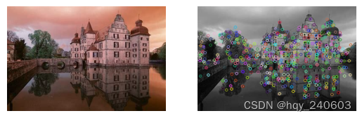
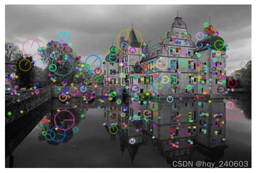
SIFT 简介（尺度不变特征变换）

Harris可以应对旋转，那么缩放呢？

–> Scale-Invariant Feature Transform (2004，D.Lowe，不列颠哥伦比亚大学)

尺度空间极值检测

进行尺度空间滤波。使用不同 $\sigma$ 值的高斯拉普拉斯算子（LoG）对图像进行卷积。具有不同 $\sigma$ 值的 LoG 可以检测不同大小的斑点。简而言之， $\sigma$ 相当于一个尺度变换因子。
例如，在上图中使用具有低 $\sigma$ 的高斯核可以检测出小的角点，而具有高 $\sigma$ 的高斯核则适合于检测大的角点。
因此，我们可以在尺度空间和二维平面中找到局部最大值 $\sigma)$ ，这意味着在 $\sigma$ 尺度中的 $(x, y)$ 处有一个潜在的特征点。

特征点定位

使用尺度空间的泰勒展开来获得潜在特征点更准确的极值位置。

指定方向

为每个特征点指定方向，以实现图像的旋转不变性。

特征点描述子

创建特征点描述子。
在关键点周围选取 16x16 的邻域。将它为 16 个 4x4 大小的子块。对于每个子块，创建包含 8 个 bin 的方向直方图。因此总共有 128 个 bin 值可用。由这 128 个形成的向量构成了特征点描述子。
除此之外，还采取了一些措施来实现对光照变化、旋转等的鲁棒性。

特征点匹配

通过识别两幅图像中距离最近的特征点来进行特征点匹配。

import numpy as np
import cv2 as cv
img = cv.imread('c:/Users/HP/Downloads/house.png')

plt.figure()  

plt.subplot(1, 2, 1)  # (rows, columns, panel number)  
plt.imshow(img)  
plt.axis('off')  # 关闭坐标轴  

gray= cv.cvtColor(img,cv.COLOR_BGR2GRAY)
sift = cv.SIFT_create()
kp = sift.detect(gray,None)
img_ = cv.drawKeypoints(gray,kp,img)
cv.imwrite('c:/Users/HP/Downloads/house_sift.png',img_)


plt.subplot(1, 2, 2)  # (rows, columns, panel number)  
plt.imshow(img_)  
plt.axis('off')  # 关闭坐标轴  



plt.show()

在这里插入图片描述

img = cv.imread('c:/Users/HP/Downloads/house.png')
img = cv.drawKeypoints(gray,kp,img,flags=cv.DRAW_MATCHES_FLAGS_DRAW_RICH_KEYPOINTS)  # 显示特征点的方向

plt.imshow(img)  
plt.axis('off')

在这里插入图片描述

现在要计算描述子，OpenCV 提供了两种方法：

如果你已经找到了特征点，可以调用 sift.compute() 来计算我们找到的特征点的描述子。例如：kp,des = sift.compute(gray,kp)。
如果你没有找到特征点，请使用函数 sift.detectAndCompute() 在一个单独步骤中直接查找特征点和描述子。

# 第二种

sift = cv.SIFT_create()
kp, des = sift.detectAndCompute(gray,None)

# 这里 kp 是一个特征点列表，des 是一个 numpy 数组，该数组大小是特征点数目乘 128

SURF 简介（加速鲁棒特性）| BRIEF（Binary Robust Independent Elementary Features）

SURF：Speeded Up Robust Features (2006，Bay，H.，Tuytelaars，T., Van Gool，L) ,顾名思义，它是 SIFT 的加速版本。

实际匹配时可能不需要所有的维度 --> BRIEF 是一种更快计算和匹配特征点描述子的方法，提供较高的识别率，除非存在大的平面内旋转。

// 由于版权保护，新版opencv不支持这个功能，，为此换版本有点太麻烦了，暂且略过；

// https://github.com/opencv/opencv/wiki/ChangeLog#version4100

features2d
- the unified framework for keypoint extraction, computing the descriptors and matching them has been introduced. The previously available and some new detectors and descriptors, like SURF, FAST, StarDetector etc. have been wrapped to be used through the framework. The key advantage of the new framework (besides the uniform API for different detectors and descriptors) is that it also provides high-level tools for image matching and textured object detection. Please, see documentation http://docs.opencv.org/modules/features2d/doc/common_interfaces_of_feature_detectors.html\ and the C++ samples:
  - descriptor_extractor_matcher.cpp – finding object in a scene using keypoints and their descriptors.
  - generic_descriptor_matcher.cpp – variation of the above sample where the descriptors do not have to be computed explicitly.
  - bagofwords_classification.cpp – example of extending the framework and using it to process data from the VOC databases: http://pascallin.ecs.soton.ac.uk/challenges/VOC/
- the newest super-fast keypoint descriptor BRIEF by Michael Calonder has been integrated by Ethan Rublee. See the sample opencv/samples/cpp/video_homography.cpp
- SURF keypoint detector has been parallelized using TBB (the patch is by imahon and yvo2m)

角点检测的 FAST 算法

之前的方法还不够快

–> FAST（Features from Accelerated Segment Test）: Machine learning for high-speed corner detection (2006/2010，Edward Rosten 和 Tom Drummond)

使用 FAST 进行特征检测
机器学习角点检测器（决策树
非最大值抑制（在相邻位置中检测到多个特征点

import numpy as np
import cv2 as cv
from matplotlib import pyplot as plt
img = cv.imread('c:/Users/HP/Downloads/chessboard3.png',0)

# Initiate FAST object with default values
fast = cv.FastFeatureDetector_create()

# find and draw the keypoints
kp = fast.detect(img,None)
img2 = cv.drawKeypoints(img, kp, None, color=(255,0,0))

# Print all default params
print( "Threshold: {}".format(fast.getThreshold()) )
print( "nonmaxSuppression:{}".format(fast.getNonmaxSuppression()) )
print( "neighborhood: {}".format(fast.getType()) )
print( "Total Keypoints with nonmaxSuppression: {}".format(len(kp)) )

# 不使用非最大值抑制
fast.setNonmaxSuppression(0)
kp = fast.detect(img,None)
print( "Total Keypoints without nonmaxSuppression: {}".format(len(kp)) )
img3 = cv.drawKeypoints(img, kp, None, color=(255,0,0))


plt.figure()  
 
plt.subplot(1, 2, 1)  # (rows, columns, panel number)  
plt.imshow(img2)  
plt.title('nonmaxSuppression')  
plt.axis('off') 
  
plt.subplot(1, 2, 2)  
plt.imshow(img3)  
plt.title('disable~')  
plt.axis('off')  
  
plt.show()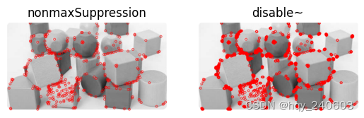

在这里插入图片描述

ORB（Oriented FAST and Rotated BRIEF）

ORB: An efficient alternative to SIFT or SURF（2011，Ethan Rublee，Vincent Rabaud，Kurt Konolige，Gary R. Bradski）

一个很好的 SIFT 和 SURF 的替代：SIFT 和 SURF 已获得专利，您应该支付它们的使用费用。但是 ORB 不是!!!

import numpy as np
import cv2 as cv
from matplotlib import pyplot as plt
img = cv.imread('c:/Users/HP/Downloads/chessboard3.png',0)

# Initiate ORB detector
orb = cv.ORB_create()

# find the keypoints with ORB
kp = orb.detect(img,None)

# compute the descriptors with ORB
kp, des = orb.compute(img, kp)

# draw only keypoints location,not size and orientation
img2 = cv.drawKeypoints(img, kp, None, color=(0,255,0), flags=0)
plt.imshow(img2)
plt.axis('off') 
plt.show()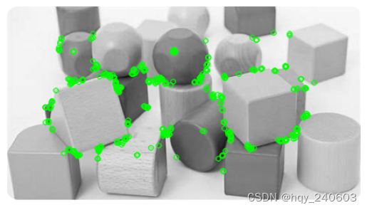

在这里插入图片描述

特征匹配

蛮力匹配的基础知识

蛮力匹配器很简单。它采用第一组中的一个特征点描述子，并使用一些距离计算与第二组中的所有其他特征点匹配。并返回距离最近的一个特征点。

对于 BF 匹配器，首先我们必须使用 cv.BFMatcher() 创建 BFMatcher 对象。
第二个参数是布尔变量 crossCheck，默认为 false。如果为 True，则 Matcher 仅返回具有值(i,j)的匹配,使得集合 A 中的第 i 个描述子具有集合 B 中的第 j 个描述子作为最佳匹配，反之亦然。
一旦创建，两个重要的方法是 BFMatcher.match() 和 BFMatcher.knnMatch()。第一个返回最佳匹配。第二种方法返回 k 个最佳匹配，其中 k 由用户指定。

对 ORB 描述子使用蛮力匹配

有一个 queryImage 和一个 trainImage，尝试使用特征匹配在 trainImage 中查找 queryImage。

使用 ORB 描述符来匹配功能。
接下来，我们使用 cv.NORM_HAMMING （因为我们使用的是 ORB）创建一个 BFMatcher 对象并且启用了 crossCheck 以获得更好的结果。
然后我们使用 Matcher.match()方法在两个图像中获得最佳匹配。
我们按照距离的升序对它们进行排序，以便最佳匹配（距离最小）出现在前面。然后画出前合适个匹配。

import numpy as np
import cv2 as cv
import matplotlib.pyplot as plt

## 图片下载地址：
## https://github.com/opencv/opencv/blob/master/samples/data/box.png
## https://github.com/opencv/opencv/blob/master/samples/data/box_in_scene.png

img1 = cv.imread('c:/Users/HP/Downloads/box.png',0)          # queryImage
img2 = cv.imread('c:/Users/HP/Downloads/box_in_scene.png',0) # trainImage

# Initiate ORB detector
orb = cv.ORB_create()
# find the keypoints and descriptors with ORB
kp1, des1 = orb.detectAndCompute(img1,None)
kp2, des2 = orb.detectAndCompute(img2,None)

# create BFMatcher object
bf = cv.BFMatcher(cv.NORM_HAMMING, crossCheck=True)
# Match descriptors.
matches = bf.match(des1,des2)
# Sort them in the order of their distance.
matches = sorted(matches, key = lambda x:x.distance)

# Draw first x matches.
img3 = cv.drawMatches(img1,kp1,img2,kp2,matches[:20], None, flags=2)  # 前20个匹配
plt.imshow(img3)
plt.axis('off') 
plt.show()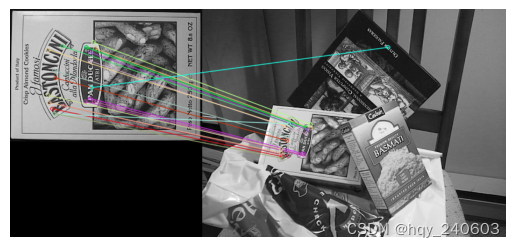

在这里插入图片描述

这个匹配器对象是什么？

matches = bf.match(des1,des2)的结果是 DMatch 对象的列表。此 DMatch 对象具有以下属性：

DMatch.distance - 描述子之间的距离。越低越好。
DMatch.trainIdx - 目标图像中描述子的索引
DMatch.queryIdx - 查询图像中描述子的索引
DMatch.imgIdx - 目标图像的索引。

对 SIFT 描述符进行蛮力匹配和比率测试

同样由于版本问题不可用，暂且略过；

// https://github.com/opencv/opencv/wiki/ChangeLog#version4100

SIFT and SURF have been moved to a separate module named nonfree to indicate possible legal issues of using those algorithms in user applications. Also, SIFT performance has been substantially improved (by factor of 3-4x).

基于 FLANN 的匹配器

FLANN 代表快速最近邻搜索包（Fast Library for Approximate Nearest Neighbors）。

它包含一系列算法，这些算法针对大型数据集中的快速最近邻搜索和高维特征进行了优化。对于大型数据集，它比 BFMatcher 工作得更快。

import numpy as np
import cv2 as cv
from matplotlib import pyplot as plt
img1 = cv.imread('c:/Users/HP/Downloads/box.png',0)          # queryImage
img2 = cv.imread('c:/Users/HP/Downloads/box_in_scene.png',0) # trainImage

# Initiate ORB detector
orb = cv.ORB_create()
# find the keypoints and descriptors with SIFT
kp1, des1 = orb.detectAndCompute(img1,None)
kp2, des2 = orb.detectAndCompute(img2,None)

# FLANN parameters
# FLANN_INDEX_KDTREE = 1
# index_params = dict(algorithm = FLANN_INDEX_KDTREE, trees = 5)
FLANN_INDEX_LSH = 6
index_params= dict(algorithm = FLANN_INDEX_LSH,
 table_number = 6, # 12
 key_size = 12, # 20
 multi_probe_level = 1) #2
#### 注意这里参数和SIFT不同

search_params = dict(checks=50)   # or pass empty dictionary
flann = cv.FlannBasedMatcher(index_params,search_params)
matches = flann.knnMatch(des1,des2,k=2)

# Need to draw only good matches, so create a mask
matchesMask = [[0,0] for i in range(len(matches))]
# ratio test as per Lowe's paper
for i,(m,n) in enumerate(matches):
    if m.distance < 0.7*n.distance:
        matchesMask[i]=[1,0]
draw_params = dict(matchColor = (0,255,0),
                   singlePointColor = (255,0,0),
                   matchesMask = matchesMask,
                   flags = 0)

img3 = cv.drawMatchesKnn(img1,kp1,img2,kp2,matches,None,**draw_params)
plt.imshow(img3,)
plt.axis('off') 
plt.show()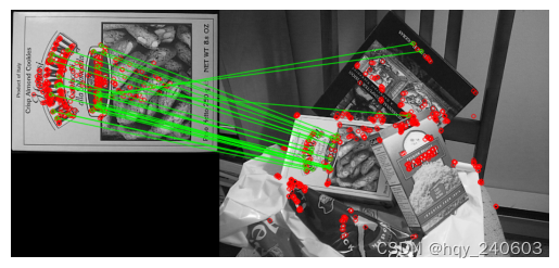

在这里插入图片描述

特征匹配+单应性查找对象

使用来自 calib3d 模块的函数，即 cv.findHomography() 。如果将两个图像中的特征点集传递给这个函数，它将找到该对象的透视变换。
然后我们可以使用 cv.perspectiveTransform() 来查找对象。它需要至少四个正确的点来找到这种变换。
使用 RANSAC 或 LEAST_MEDIAN（可以由标志位决定）。因此，提供正确估计的良好匹配称为内点，剩余称为外点。 cv.findHomography() 返回一个指定了内点和外点的掩模。

import numpy as np
import cv2 as cv
from matplotlib import pyplot as plt




#### 首先，在图像中找到 ORB 特征并应用比率测试来找到最佳匹配。


MIN_MATCH_COUNT = 10

img1 = cv.imread('c:/Users/HP/Downloads/box.png',0)          # queryImage
img2 = cv.imread('c:/Users/HP/Downloads/box_in_scene.png',0) # trainImage

# Initiate ORB detector
orb = cv.ORB_create()
# find the keypoints and descriptors with SIFT
kp1, des1 = orb.detectAndCompute(img1,None)
kp2, des2 = orb.detectAndCompute(img2,None)

# FLANN parameters
# FLANN_INDEX_KDTREE = 1
# index_params = dict(algorithm = FLANN_INDEX_KDTREE, trees = 5)
FLANN_INDEX_LSH = 6
index_params= dict(algorithm = FLANN_INDEX_LSH,
 table_number = 6, # 12
 key_size = 12, # 20
 multi_probe_level = 1) #2
#### 注意这里参数和SIFT不同

search_params = dict(checks = 50)
flann = cv.FlannBasedMatcher(index_params, search_params)
matches = flann.knnMatch(des1,des2,k=2)
# store all the good matches as per Lowe's ratio test.
good = []
for m,n in matches:
    if m.distance < 0.7*n.distance:
        good.append(m)




#### 现在设置至少 10 个匹配（由 MIN_MATCH_COUNT 定义）时才查找目标对象。否则只显示一条消息，说明没有足够的匹配。
#    如果找到足够的匹配则提取两个图像中匹配的特征点的位置，传入函数中以找到透视变换。
#    用这个 3x3 变换矩阵将 queryImage 中的角点转换为 trainImage 中的对应点。然后绘制出来。


if len(good)>MIN_MATCH_COUNT:
    src_pts = np.float32([ kp1[m.queryIdx].pt for m in good ]).reshape(-1,1,2)
    dst_pts = np.float32([ kp2[m.trainIdx].pt for m in good ]).reshape(-1,1,2)
    M, mask = cv.findHomography(src_pts, dst_pts, cv.RANSAC,5.0)
    matchesMask = mask.ravel().tolist()
    h,w= img1.shape
    pts = np.float32([ [0,0],[0,h-1],[w-1,h-1],[w-1,0] ]).reshape(-1,1,2)
    dst = cv.perspectiveTransform(pts,M)
    img2 = cv.polylines(img2,[np.int32(dst)],True,255,3, cv.LINE_AA)
else:
    print( "Not enough matches are found - {}/{}".format(len(good), MIN_MATCH_COUNT) )
    matchesMask = None




#### 最后，我们绘制内点（如果成功找到对象）或匹配特征点（如果失败）。


draw_params = dict(matchColor = (0,255,0), # draw matches in green color
                   singlePointColor = None,
                   matchesMask = matchesMask, # draw only inliers
                   flags = 2)
img3 = cv.drawMatches(img1,kp1,img2,kp2,good,None,**draw_params)
plt.imshow(img3, 'gray')
plt.axis('off') 
plt.show()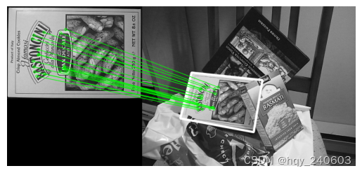