视频deep_thoughts
论文https://arxiv.org/abs/2010.02502
参考https://blog.csdn.net/weixin_47748259/article/details/137018607

DDPM生成过程就是把每一步都看作高斯分布的形式，所以采样过程和前向加噪过程的链条长度是一致的。DDIM就是在思考能不能够加速这个采样过程。

DDPM-马尔科夫扩散

DDPM原理

DDIM论文中的${\alpha }_t$,其实是DDPM论文中的$\overline{\alpha }$,所以DDIM论文前向过程${\beta }_t=1-\frac{{\alpha }_t}{{\alpha }_{t-1}}$本博客中为了统一把原DDIM论文对应的$\alpha$都写成$\overline{\alpha }$,笔者可能有漏掉的地方，请大家多多指正！

• 在DDPM中，扩散过程(前向过程)定义为一个马尔卡夫链：
  $$q(x_{1:T}|x_0):=\prod _{t=1}^{T}q(x_t|x_{t-1}),\text{where }q(x_t|x_{t-1}):=\mathcal{N}\left(\sqrt{1-{\beta }_t}{x}_{t-1},{\beta }_{t}I\right)$$
  扩散过程的一个重要特性是可以直接用$x_0$来对任意的$x_t$进行采样：
  $$q({\mathbf{x}}_t|{\mathbf{x}}_0):=\int q({\mathbf{x}}_{1:t}|{\mathbf{x}}_0)\mathrm{d}{\mathbf{x}}_{1:(t-1)}=\mathcal{N}({\mathbf{x}}_t;\sqrt{{\overline{\alpha }}_t}{\mathbf{x}}_0,(1-{\overline{\alpha }}_t)\mathbf{I});$$
  $x_t$可以表示为$x_0$和噪声变量$\epsilon$的线性组合
  $$x_t=\sqrt{{\bar{\alpha }}_t}{x}_0+\sqrt{1-{\bar{\alpha }}_t}ϵ,\mathrm{where}ϵ\sim \mathcal{N}(0,\mathbf{I})$$

• DDPM的反向过程也定义为一个马尔卡夫链：
  $$p_{\theta }(x_0)=\int p_{\theta }(x_{0:T})\mathrm{d}{x}_{1:T},\mathrm{where}{p}_{\theta }(x_{0:T}):=p_{\theta }(x_T)\prod _{t=1}^T{p}_{\theta }^{(t)}(x_{t-1}|x_t)$$
  反向过程使用神经网络$p_{\theta }\left(x_{t-1}\mid x_t\right)$拟合真实的分布$q(x_t-1\mid x_t)$。

• DDPM的目标函数：最大化变分下界来学习参数$\theta$以拟合数据分布
  $$\underset{\theta }{\max }{\mathbb{E}}_{q({\mathbf{x}}_0)}[\log p_{\theta }({\mathbf{x}}_0)]\le \underset{\theta }{\max }{\mathbb{E}}_{q({\mathbf{x}}_0,{\mathbf{x}}_1,...,{\mathbf{x}}_T)}\left[\log p_{\theta }({\mathbf{x}}_{0:T})-\log q({\mathbf{x}}_{1:T}|{\mathbf{x}}_0)\right]$$
  通过一系列的推导可以得到目标函数的简化版：
  $$L_{\gamma }({ϵ}_{\theta }):=\sum _{t=1}^T{\gamma }_t{\mathbb{E}}_{{\mathbf{x}}_0\sim q({\mathbf{x}}_0),{ϵ}_t\sim \mathcal{N}(0,\mathbf{I})}\left[{\Vert {ϵ}_{\theta }^{(t)}(\sqrt{{\overline{\alpha }}_t}{x}_0+\sqrt{1-{\overline{\alpha }}_t}{ϵ}_t)-{ϵ}_t\Vert }_2^2\right]$$

  • ${\gamma }_t$是系数，当${\gamma }_t=1$时，这个目标函数其实也是分数匹配模型 (score matching)的目标函数。
  • 目标函数仅仅取决于边缘分布$q(x_t|x_0)$，而不是取决于联合分布$q(x_{1:T}|x_0)$。在推导出DDPM的$L_{simple}$的过程中，没有用到联合分布$q(x_{1:T}|x_0)$，只是基于贝叶斯公式和$q(x_t|x_{t-1},x_0)$、$q(x_t|x_0)$表达式。

DDPM缺点

DDPM的前向加噪过程需要进行多步马尔科夫链采样，如果步数较大（比如1000步），那么在去噪过程中需要使用Unet生成噪声，并进行相同数量的步数（1000步）来去除噪声。DDPM过程的一个问题是在训练后生成图像的速度过慢。
GAN模型的采样质量是比较高的，但是GAN需要在优化策略上以及结构设计方面做出非常具体的选择，并且容易陷入到一种模式中去，产出的多样性较差。
DDPM和NCSN（噪声条件评分网络）具有产生与GAN相当的样本的能力，而无需进行对抗性训练。他们首先会对样本加噪，然后通过马尔科夫链对其逆过程进行建模，该链从白噪声开始，逐渐将其降噪为图像。这种生成马尔可夫链过程要么基于郎之万动力学，要么通过反转逐渐将图像转化为噪声的前向扩散过程获得。这些模型的缺点在于需要多次迭代才能生成高质量的样本。

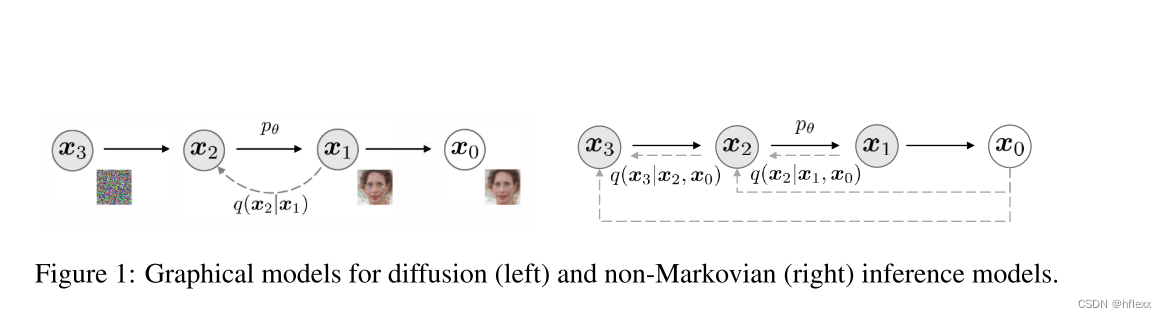
DDIM-非马尔科夫的扩散

非马尔科夫链的前向扩散过程

$$\begin{array}{rl}{q}_{\sigma }({\mathbf{x}}_{1:T}|{\mathbf{x}}_0):& =q_{\sigma }({\mathbf{x}}_T|{\mathbf{x}}_0)\prod _{t=2}^T{q}_{\sigma }({\mathbf{x}}_{t-1}|{\mathbf{x}}_t,{\mathbf{x}}_0)\\ \text{where }{q}_{\sigma }({\mathbf{x}}_T|{\mathbf{x}}_0)& =\mathcal{N}(\sqrt{{\bar{\alpha }}_T}{\mathbf{x}}_0,(1-{\bar{\alpha }}_T)\mathbf{I})\end{array}$$
$$\boxed{q_{\sigma }({\mathbf{x}}_{t-1}|{\mathbf{x}}_t,{\mathbf{x}}_0)=\mathcal{N}\left(\sqrt{{\bar{\alpha }}_{t-1}}{\mathbf{x}}_0+\sqrt{1-{\bar{\alpha }}_{t-1}-{\sigma }_t^2}\cdot \frac{{\mathbf{x}}_t-\sqrt{{\bar{\alpha }}_t}{\mathbf{x}}_0}{\sqrt{1-{\bar{\alpha }}_t}},{\sigma }_t^2\mathbf{I}\right)\text{for }t>1}$$

• 一个新的推理分布族 Q， σ为超参数

• $q_{\sigma }(x_{1:T}|x_0)$：这是给定初始数据 $x_0$ 时，整个状态序列 $x_{1:T}$ 的联合概率分布。这个分布是由一系列的条件概率分布组成的，它描述了一个从 $x_0$ 开始的非马尔可夫推理过程。

• $q_{\sigma }(x_T|x_0)$：这是在时间步 $T$ 时条件概率分布，它描述了从 $x_0$ 到 $x_T$ 的直接关系。在许多DDPMs的实现中，$x_T$ 通常是一个高斯分布，其均值为零，表示在最后一步中，数据完全转化为噪声。

• ${\prod }_{t=2}^T{q}_{\sigma }(x_{t-1}|x_t,x_0)$：这是一个条件概率分布的乘积，它表示从 $x_0$ 经过中间状态 $x_1,x_2,...,x_{T-1}$ 到 $x_T$ 的过程。与标准的马尔可夫链不同，这里的每个 $q_{\sigma }(x_{t-1}|x_t,x_0)$ 可能同时依赖于 $x_t$ 和 $x_0$，因此不是纯粹的马尔可夫链。

• $\sigma$：这是一个参数，它控制了推理过程的非马尔可夫性质的程度。不同的 $\sigma$ 值可以导致不同的推理和生成过程，但它们可以使用相同的神经网络参数 $\theta$ 来实现，因为它们共享相同的边缘分布 $q(x_t|x_0)$。当 σ → 0 时，我们达到了一种极端情况，只要我们在某个 t 内观察 x0 和 xt，那么$x_{t-1}$ 就变得已知并固定

逆向生成过程与目标函数

这一节的核心内容是定义了一个与非马尔可夫前向过程相匹配的生成过程，并展示了如何通过变分推断来优化模型参数。

1. 生成过程的定义：作者定义了一个生成过程 $p_{\theta }(x_{0:T})$，该过程利用了非马尔可夫前向过程 $q_{\sigma }(x_{t-1}|x_t,x_0)$ 的知识。在这个生成过程中，给定一个噪声观测 $x_t$，模型首先预测对应的 $x_0$，然后通过逆条件分布 $q_{\sigma }(x_{t-1}|x_t,x_0)$ 获得 $x_{t-1}$ 的样本。
   重新编写$x_t=\sqrt{\overline{a_t}}{x}_0+\sqrt{1-\overline{a_t}}ϵ\text{，}whereϵ\sim N(0,1)$,即给定$x_t$后$x_0$的预测 ：
   $$\begin{gathered} x_t=\sqrt{\overline{a_t}}{x}_0+\sqrt{1-\overline{a_t}}ϵ\text{，}whereϵ\sim N(0,1) \\ \Downarrow \\ 重新编写后 \\ {f}_{\theta }^{(t)}({\mathbf{x}}_t):=({\mathbf{x}}_t-\sqrt{1-{\bar{\alpha }}_t}\cdot {ϵ}_{\theta }^{(t)}({\mathbf{x}}_t))/\sqrt{{\bar{\alpha }}_t} \end{gathered}$$

   • ${ϵ}_{\theta }^{(t)}(x_t)$:predict ${ϵ}_t$ from $x_t$,用于预测在时间步 t时添加到原始数据中的噪声，不用知道$x_0$
   • 由$x_t=\sqrt{\overline{a_t}}{x}_0+\sqrt{1-\overline{a_t}}ϵ（ϵ\sim N(0,1)）$重新编写而来
     定义具有固定先验分布（a fixed prior）的生成过程

$$p_{\theta }(x_T)=N(0,I)$$$${p}_{\theta }^{(t)}({\mathbf{x}}_{t-1}|{\mathbf{x}}_t)=\{\begin{array}{ll}\mathcal{N}(f_{\theta }^{(1)}({\mathbf{x}}_1),{\sigma }_1^2\mathbf{I})& \text{if }t=1\\ q_{\sigma }({\mathbf{x}}_{t-1}|{\mathbf{x}}_t,f_{\theta }^{(t)}({\mathbf{x}}_t))& \text{otherwise,}\end{array}$$

• $q_{\sigma }({\mathbf{x}}_{t-1}|{\mathbf{x}}_t,{\mathbf{x}}_0)=\mathcal{N}\left(\sqrt{{\bar{\alpha }}_{t-1}}{\mathbf{x}}_0+\sqrt{1-{\bar{\alpha }}_{t-1}-{\sigma }_t^2}\cdot \frac{{\mathbf{x}}_t-\sqrt{{\bar{\alpha }}_t}{\mathbf{x}}_0}{\sqrt{1-{\bar{\alpha }}_t}},{\sigma }_t^2\mathbf{I}\right)$

• $p_{\theta }(x_T)=N(0,I)$定义了在时间步 $T$时的先验分布，即在扩散过程的最后，数据$x_T$ 被假设为一个以零为均值（即完全噪声）和单位方差（即没有额外噪声）的高斯分布。这意味着在扩散过程的开始，数据$x_T$ 是完全未知的，这为生成过程提供了一个起点。

• $\mathcal{N}(\mu ,\Sigma )$表示均值为$\mu$和协方差矩阵为$\Sigma$的多变量高斯分布。

• $I$ 是单位矩阵。

• ${\sigma }_1^2$ 是 t=1 时引入的固定方差项,在 t = 1 的情况下添加一些高斯噪声，以确保生成过程在任何地方都得到支持

• $f_{\theta }^{(t)}({\mathbf{x}}_t)$ 是在时间步 $t$的去噪函数，用于预测原始数据 $x_0$

2. 变分推断目标：作者提出了一个变分推断目标 $J_{\sigma }({ϵ}_{\theta })$，用于优化模型参数 $\theta$。这个目标函数是一个关于 ${ϵ}_{\theta }$ 的泛函，它涉及到对生成过程和前向过程的对数概率的差值的期望。

$$\begin{gathered} J_{\sigma }({ϵ}_{\theta }):={\mathbb{E}}_{x_{0:T}\sim q_{\sigma }(x_{0:T})}[\log q_{\sigma }(x_{1:T}|x_0)-\log p_{\theta }(x_{0:T})]= \\ {\mathbb{E}}_{{\mathbf{x}}_{0:T}\sim q_{\sigma }({\mathbf{x}}_{0:T})}\left[\log q_{\sigma }({\mathbf{x}}_T|{\mathbf{x}}_0)+\sum _{t=2}^T\log q_{\sigma }({\mathbf{x}}_{t-1}|{\mathbf{x}}_t,{\mathbf{x}}_0)-\sum _{t=1}^T\log p_{\theta }^{(t)}({\mathbf{x}}_{t-1}|{\mathbf{x}}_t)-\log p_{\theta }({\mathbf{x}}_T)\right] \end{gathered}$$

• 如果模型${ϵ}_{\theta }^{(t)}$的参数$\theta$在不同的时间步$t$之间不共享，那么对于${ϵ}_{\theta }$的最优解将不依赖于权重 $\gamma$这是因为全局最优解可以通过分别最大化目标函数中的每一项来实现。

• $L_{\gamma }$的这种性质，使用$L_1$即$\gamma =1$的情况）作为变分下界的替代目标函数在DDPMs中是合理的。这意味着即使在不同的时间步使用不同的参数，优化$L_1$也能得到一个好的解。

• $J_{\sigma }$与 $L_{\gamma }$的等价性：根据定理 1，对于所有的$\sigma >0$,存在权重$\gamma$和常数$C$使得$J_{\sigma }=L_{\gamma }+C$ 这表明$J_{\sigma }$ 和$L_{\gamma }$是等价的，因此$J_{\sigma }$的最优解也与$L_1$的最优解相同。

• $L_1$作为$J_{\sigma }$的替代目标**：如果模型${ϵ}_{\theta }$中的参数在不同的$t$之间不共享，那么 Ho 等人（2020）使用的$L_1$目标函数也可以用作变分目标$J_{\sigma }$的替代目标函数。这意味着在这种情况下，可以使用$L_1$来训练模型，而不需要为每个$\sigma$选择不同的权重$\gamma$。

• 这意味着不需要对模型进行重新训练，只需改变非马尔可夫过程的参数 $\sigma$ 即可。

非马尔科夫扩散逆过程的采样

DDPM的生成过程实际上是模拟加噪过程的逆过程。由于DDPM的加噪过程是以高斯分布的形式进行多步加噪，因此生成过程就是把每一步都看作高斯分布的形式，所以采样过程和前向加噪过程的链条长度是一致的。DDIM就是在思考能不能够加速这个采样过程。

对比非马尔科夫扩散后验分布与DDPM马尔科夫扩散的后验分布

• DDPM马尔科夫扩散的后验分布为：
  $$\begin{array}{rl}q({\mathbf{x}}_{t-1}|{\mathbf{x}}_t,{\mathbf{x}}_0)& =\mathcal{N}({\mathbf{x}}_{t-1};{\tilde{\mathbf{\mu }}}_t({\mathbf{x}}_t,{\mathbf{x}}_0),{\tilde{\beta }}_t\mathbf{I}),\\ \mathrm{where}{\tilde{\mu }}_t({\mathbf{x}}_t,{\mathbf{x}}_0)& :=\frac{\sqrt{{\bar{\alpha }}_{t-1}}{\beta }_t}{1-{\bar{\alpha }}_t}{\mathbf{x}}_0+\frac{\sqrt{{\alpha }_t}(1-{\bar{\alpha }}_{t-1})}{1-{\bar{\alpha }}_t}{\mathbf{x}}_t\mathrm{and}{\tilde{\beta }}_t:=\frac{1-{\bar{\alpha }}_{t-1}}{1-{\bar{\alpha }}_t}\end{array}$$
• DDIM的后验分布为：
  $$\begin{gathered} q_{\sigma }({\mathbf{x}}_T|{\mathbf{x}}_0)=\mathcal{N}(\sqrt{{\bar{\alpha }}_T}{\mathbf{x}}_0,(1-{\bar{\alpha }}_T)\mathbf{I})\text{ and for all }t>1, \\ {q}_{\sigma }({\mathbf{x}}_{t-1}|{\mathbf{x}}_t,{\mathbf{x}}_0)=\mathcal{N}\left(\sqrt{{\bar{\alpha }}_{t-1}}{\mathbf{x}}_0+\sqrt{1-{\bar{\alpha }}_{t-1}-{\sigma }_t^2}\cdot \frac{{\mathbf{x}}_t-\sqrt{{\bar{\alpha }}_t}{\mathbf{x}}_0}{\sqrt{1-\bar{\alpha }{\mathbf{x}}_t}},{\sigma }_t^2\mathbf{I}\right) \end{gathered}$$
  对比可知，DDIM中的后验分布相较于DDPM的后验分布多了一个超参数${\sigma }_t$,其决定了扩散模型的后验分布，同时也就决定了扩散逆过程的采样。

超参数$\sigma$的选择
以$L_1$为目标，可以生成DDIM对应的由参数化σ对应的无马尔科夫链过程。本质上可以使用预训练的 DDPM 模型作为新目标的解决方案，并专注于寻找一种生成过程，通过改变 σ 来更好地生成符合我们需求的样本。
$${\sigma }_{{\tau }_i}(\eta )=\eta \sqrt{(1-{\alpha }_{{\tau }_{i-1}})/(1-{\alpha }_{{\tau }_i})}\sqrt{1-{\alpha }_{{\tau }_i}/{\alpha }_{{\tau }_{i-1}}}$$

可以推导出以下方式从样本$x_t$生成$x_{t-1}$

$$\{\begin{array}{l}{p}_{\theta }(x_T)=N(0,I)\\ p_{\theta }^{(t)}({\mathbf{x}}_{t-1}|{\mathbf{x}}_t)=\{\begin{array}{ll}\mathcal{N}(f_{\theta }^{(1)}({\mathbf{x}}_1),{\sigma }_1^2\mathbf{I})& \text{if }t=1\\ q_{\sigma }({\mathbf{x}}_{t-1}|{\mathbf{x}}_t,f_{\theta }^{(t)}({\mathbf{x}}_t))& \text{otherwise}\end{array}\\ f_{\theta }^{(t)}({\mathbf{x}}_t):=({\mathbf{x}}_t-\sqrt{1-{\bar{\alpha }}_t}\cdot {ϵ}_{\theta }^{(t)}({\mathbf{x}}_t))/\sqrt{{\bar{\alpha }}_t}\\ \\ q_{\sigma }({\mathbf{x}}_{t-1}|{\mathbf{x}}_t,{\mathbf{x}}_0)=\mathcal{N}\left(\sqrt{{\bar{\alpha }}_{t-1}}{\mathbf{x}}_0+\sqrt{1-{\bar{\alpha }}_{t-1}-{\sigma }_t^2}\cdot \frac{{\mathbf{x}}_t-\sqrt{{\bar{\alpha }}_t}{\mathbf{x}}_0}{\sqrt{1-{\bar{\alpha }}_t}},{\sigma }_t^2\mathbf{I}\right)\end{array}$$

$$\Downarrow$$
$${\mathbf{x}}_{t-1}=\sqrt{{\bar{\alpha }}_{t-1}}\underset{\text{“predicted }{\mathbf{x}}_0\text{”}}{\underbrace{\left(\frac{{\mathbf{x}}_t-\sqrt{1-{\bar{\alpha }}_t}{ϵ}_{\theta }^{(t)}({\mathbf{x}}_t)}{\sqrt{{\bar{\alpha }}_t}}\right)}}+\underset{\text{“direction pointing to }{\mathbf{x}}_t\text{”}}{\underbrace{\sqrt{1-{\bar{\alpha }}_{t-1}-{\sigma }_t^2}\cdot {ϵ}_{\theta }^{(t)}({\mathbf{x}}_t)}}+\underset{\text{random noise}}{\underbrace{{\sigma }_t{ϵ}_t}}$$

respacing：加速采样的技巧
考虑不从完整的时间序列$x_{1:T}$上采样，而是从它的一个子集上采样： { x τ 1 , . . . , x τ s } \{x_{\tau_1},...,x_{\tau_s}\} {xτ1​​,...,xτs​​}，其中$s<t$。进而就有：$q(x_{{\tau }_i}|x_0)=N(\sqrt{{\alpha }_{{\tau }_i}}{x}_0,(1-{\alpha }_{{\tau }_i})I)$。因此原始的采样需要经T步，而respacing技巧下只需要经过S步，实现加速采样。对比结果发现，在ddim模型上使用respacing技巧可以保证采样速度更快的情况下图像质量更高。

$q_{\sigma }$推导

根据b站up主“大白话”所推导出来的，这个方便理解一些
对于一个已经训练好的DDPM，只需要对采样公式做简单的修改，模型就能在去噪时「跳步骤」，在一步去噪迭代中直接预测若干次去噪后的结果。

$$p_{\theta }(x_T)=N(0,I)$$$${p}_{\theta }^{(t)}({\mathbf{x}}_{t-1}|{\mathbf{x}}_t)=\{\begin{array}{ll}\mathcal{N}(f_{\theta }^{(1)}({\mathbf{x}}_1),{\sigma }_1^2\mathbf{I})& \text{if }t=1\\ q_{\sigma }({\mathbf{x}}_{t-1}|{\mathbf{x}}_t,f_{\theta }^{(t)}({\mathbf{x}}_t))& \text{otherwise,}\end{array}$$
$$\Downarrow$$
$${\mathbf{x}}_{t-1}=\sqrt{{\bar{\alpha }}_{t-1}}\underset{\text{“predicted }{\mathbf{x}}_0\text{”}}{\underbrace{\left(\frac{{\mathbf{x}}_t-\sqrt{1-{\bar{\alpha }}_t}{ϵ}_{\theta }^{(t)}({\mathbf{x}}_t)}{\sqrt{{\bar{\alpha }}_t}}\right)}}+\underset{\text{“direction pointing to }{\mathbf{x}}_t\text{”}}{\underbrace{\sqrt{1-{\bar{\alpha }}_{t-1}-{\sigma }_t^2}\cdot {ϵ}_{\theta }^{(t)}({\mathbf{x}}_t)}}+\underset{\text{random noise}}{\underbrace{{\sigma }_t{ϵ}_t}}$$

• ${ϵ}_t$:与$x_t$无关的标准高斯分布噪声
• ${\alpha }_0$:定义为1
• 不同的 σ 值选择会导致不同的生成过程，
• 使用相同的模型${ϵ}_{\theta }$，因此无需重新训练模型
• 当${\sigma }_t=\sqrt{(1-{\bar{\alpha }}_{t-1})/(1-{\bar{\alpha }}_t)}\sqrt{1-{\bar{\alpha }}_t/{\bar{\alpha }}_{t-1}}$时，生成过程就是之前的DDPM模型了。
• 当当${\sigma }_t=0$时，随机噪声${ϵ}_t$系数变成0，这使模型变成一种隐式概率模型（样本是从潜在变量通过一个固定的程序生成的,从$x_T$到$x_0$），在这种情况下除了t=1的情况，其他情况下，给定$x_0,x_t$后，前向过程是确定性的

设$P(x_{t-1}|x_t,x_0)$满足如下正态分布，即：
$$\begin{gathered} P(x_{t-1}|x_t,x_0)\sim N(k{x}_0+m{x}_t,{\sigma }^2),\text{where }ϵ\sim N(0,1) \\ \Downarrow \\ \text{即}:x_{t-1}=k{x}_o+m{x}_t+\sigma ϵ\text{\hspace{1em}(2)} \end{gathered}$$

又因为前向的加噪过程满足：
$$x_t=\sqrt{\overline{a_t}}{x}_0+\sqrt{1-\overline{a_t}}ϵ\text{ where }ϵ\sim N(0,1)\text{\hspace{1em}(3)}$$

合并上面（1）（2），有：
$$x_{t-1}=k{x}_o+m{x}_t+\sigma ϵ=k{x}_0+m[\sqrt{{\bar{a}}_t}{x}_0+\sqrt{1-{\bar{a}}_t}ϵ]+\sigma ϵ\text{\hspace{1em}(4)}$$

合并$x_0$的系数有：
$$\begin{array}{rl}& x_{t-1}=(k+m\sqrt{{\bar{a}}_t})x_0+{ϵ}^{\prime }\\ & \text{where }{ϵ}^{\prime }\sim M(0,m^2(1-{\bar{a}}_t)+{\sigma }^2)\end{array}\text{\hspace{1em}(5)}$$
由DDPM中可知在前向过程中$x_{t-1}可以由$：
$$x_{t-1}=\sqrt{{\bar{a}}_{t-1}}{x}_0+\sqrt{1-{\bar{a}}_{t-1}}ϵ\text{\hspace{1em}(6)}$$
通过式(4)(5)的$x_{t-1}$服从的概率分布可知：
$$\begin{gathered} k+m\sqrt{{\bar{a}}_t}=\sqrt{{\bar{a}}_{t-1}} \\ {m}^2(1-{\bar{a}}_t)+{\sigma }^2=1-{\bar{a}}_{t-1}\text{\hspace{1em}(7)} \end{gathered}$$
由式(6)两个式子可解出：

$$\{\begin{array}{rl}m& =\frac{\sqrt{1-{\alpha }_{t-1}^{-}-{\sigma }^2}}{\sqrt{1-\overline{{\alpha }_t}}}\\ k& =\sqrt{{\alpha }_{t-1}^{-}}-\frac{\sqrt{1-{\alpha }_{t-1}^{-}-{\sigma }^2}}{\sqrt{1-\overline{{\alpha }_t}}}\sqrt{\overline{{\alpha }_t}}\end{array}$$
将m，k带入到$P(x_{t-1}|x_t,x_0)$中，可得：
$$\begin{gathered} P(x_{t-1}|x_t,x_0)\sim N(k{x}_0+m{x}_t,{\sigma }^2),\text{where }ϵ\sim N(0,1) \\ \Downarrow \\ \begin{array}{rl}& P(x_{t-1}|x_t,x_0)\sim N((\sqrt{{\alpha }_{t-1}^{-}}-\frac{\sqrt{1-{\alpha }_{t-1}^{-}-{\sigma }^2}}{\sqrt{1-{\bar{\alpha }}_t}}\sqrt{{\bar{\alpha }}_t})x_0+(\frac{\sqrt{1-{\alpha }_{t-1}^{-}-{\sigma }^2}}{\sqrt{1-{\bar{\alpha }}_t}})x_t,{\sigma }^2)\\ & \sim N(\sqrt{{\alpha }_{t-1}^{-}}{x}_0+\sqrt{1-{\alpha }_{t-1}^{-}-{\sigma }^2}\frac{x_t-\sqrt{{\bar{\alpha }}_t}{x}_0}{\sqrt{1-{\bar{\alpha }}_t}},{\sigma }^2)\end{array} \end{gathered}$$

依旧可以使用$x_t,x_0$的关系式把$x_0$去掉,代入$x_t=\sqrt{\overline{a_t}}{x}_0+\sqrt{1-\overline{a_t}}{ϵ}_t$:后

从$P(x_{t-1}|x_t,x_0)$的概率分布采样可得到：
$$\boxed{x_{t-1}=\sqrt{{\alpha }_{t-1}^{-}}(\frac{x_t-\sqrt{1-\overline{{\alpha }_t}}{ϵ}_t}{\sqrt{\overline{{\alpha }_t}}})+\sqrt{1-{\alpha }_{t-1}^{-}-{\sigma }^2}{ϵ}_t+{\sigma }^2ϵ}$$

• $ϵ$是从标准正太分布中，随机采样得到；
• ${ϵ}_t$ 是和DDPM一样，使用神经网络训练而来的；
• $x_t$是输入
• ${\bar{a}}_{t-1}$ 和${\bar{a}}_t$ 是事先定义好的。

至此，我们就只需要讨论$\sigma$这个参数了，论文中通过实验得到：
$${\sigma }_{{\tau }_i}(\eta )=\eta \sqrt{(1-{\bar{\alpha }}_{{\tau }_{i-1}})/(1-{\bar{\alpha }}_{{\tau }_i})}\sqrt{1-{\bar{\alpha }}_{{\tau }_i}/{\bar{\alpha }}_{{\tau }_{i-1}}}$$

• $\eta$=1,对应ddim
• $\eta$=0,对应ddpm

DDIM核心代码

参考openai的improved-diffusion原码

ddim采样

DDIM（Denoising Diffusion Probabilistic Models）进行采样。主要包括：

• ddim_sample: 使用DDIM从模型中对$x_{t-1}$进行采样。

• ddim_reverse_sample: 使用DDIM反向ODE（Ordinary Differential Equation）从模型中对$x_{t+1}$进行采样。

• ddim_sample_loop: 使用DDIM从模型生成样本。

• ddim_sample_loop_progressive: 使用DDIM从模型生成样本，并逐步生成每个DDIM时间步骤的中间样本。

ddim_sample从模型中使用DDIM对 x_{t-1} 进行采样，利用
$x_{t-1}=\sqrt{{\alpha }_{t-1}^{-}}(\frac{x_t-\sqrt{1-\overline{{\alpha }_t}}{ϵ}_t}{\sqrt{\overline{{\alpha }_t}}})+\sqrt{1-{\alpha }_{t-1}^{-}-{\sigma }^2}{ϵ}_t+{\sigma }^2ϵ$得到$x_{t-1}$和$x_t=\sqrt{{\alpha }_t}{x}_0+\sqrt{1-{\alpha }_t}ϵ,(ϵ\sim \mathcal{N}(0,\mathbf{I}))$得到对应的$ϵ$

def ddim_sample(
    self,
    model,
    x,
    t,
    clip_denoised=True,
    denoised_fn=None,
    model_kwargs=None,
    eta=0.0,
):
    """
    使用DDIM从模型中对 x_{t-1} 进行采样。

    与 p_sample() 的用法相同。
    """
    # 使用 p_mean_variance 函数计算均值和方差
    #得到前一时刻的均值和方差
    out = self.p_mean_variance(
        model,
        x,
        t,
        clip_denoised=clip_denoised,
        denoised_fn=denoised_fn,
        model_kwargs=model_kwargs,
    )
    # Usually our model outputs epsilon, but we re-derive it
    # in case we used x_start or x_prev prediction.
    
    '''
    def _predict_eps_from_xstart(self, x_t, t, pred_xstart):
        return (
            _extract_into_tensor(self.sqrt_recip_alphas_cumprod, t, x_t.shape) * x_t- pred_xstart
        ) / _extract_into_tensor(self.sqrt_recipm1_alphas_cumprod, t, x_t.shape)
     函数_predict_eps_from_xstart用于反推出epsilon
     pred_xstart是预测的起始点
        '''
    # _predict_eps_from_xstart用于根据x_t,t和反推出epsilon
    eps = self._predict_eps_from_xstart(x, t, out["pred_xstart"])
 
    alpha_bar = _extract_into_tensor(self.alphas_cumprod, t, x.shape)
    alpha_bar_prev = _extract_into_tensor(self.alphas_cumprod_prev, t, x.shape)

    # 计算用于注入噪声的 sigma
    sigma = (
        eta
        * th.sqrt((1 - alpha_bar_prev) / (1 - alpha_bar))
        * th.sqrt(1 - alpha_bar / alpha_bar_prev)
    )
    #利用DDIM论文的公式12进行计算
    noise = th.randn_like(x)
    # 计算均值预测
    mean_pred = (
        out["pred_xstart"] * th.sqrt(alpha_bar_prev)
        + th.sqrt(1 - alpha_bar_prev - sigma ** 2) * eps
    )
    nonzero_mask = (
    #t不等于0的时候需要有噪音，t等于0即最后一个时刻时直接输出均值
    #最后一个时刻直接预测的是期望值
        (t != 0).float().view(-1, *([1] * (len(x.shape) - 1)))
    )
    # 生成样本，即重采样得到的结果
    sample = mean_pred + nonzero_mask * sigma * noise
    return {"sample": sample, "pred_xstart": out["pred_xstart"]}

ddim_reverse_sample使用DDIM反向ODE从模型中对 $x_{t+1}$ 进行采样。

def ddim_reverse_sample(
    self,
    model,
    x,
    t,
    clip_denoised=True,
    denoised_fn=None,
    model_kwargs=None,
    eta=0.0,
):
    """
    使用DDIM反向ODE从模型中对 x_{t+1} 进行采样。
    """
    # 确保 eta 为 0 用于反向ODE
    assert eta == 0.0, "Reverse ODE only for deterministic path"
    # 使用 p_mean_variance 函数计算均值和方差
    out = self.p_mean_variance(
        model,
        x,
        t,
        clip_denoised=clip_denoised,
        denoised_fn=denoised_fn,
        model_kwargs=model_kwargs,
    )
    # 计算用于采样的 epsilon
    eps = (
        _extract_into_tensor(self.sqrt_recip_alphas_cumprod, t, x.shape) * x
        - out["pred_xstart"]
    ) / _extract_into_tensor(self.sqrt_recipm1_alphas_cumprod, t, x.shape)
    alpha_bar_next = _extract_into_tensor(self.alphas_cumprod_next, t, x.shape)

    # 计算均值预测
    mean_pred = (
        out["pred_xstart"] * th.sqrt(alpha_bar_next)
        + th.sqrt(1 - alpha_bar_next) * eps
    )

    return {"sample": mean_pred, "pred_xstart": out["pred_xstart"]}

ddim_sample_loop于在模型中使用DDIM技术进行采样

def ddim_sample_loop(
        self,
        model,
        shape,
        noise=None,
        clip_denoised=True,
        denoised_fn=None,
        model_kwargs=None,
        device=None,
        progress=False,
        eta=0.0,
    ):
        """
        从模型中使用DDIM生成样本。

        与 p_sample_loop() 的用法相同。
        """
        final = None
        for sample in self.ddim_sample_loop_progressive(
            model,
            shape,
            noise=noise,
            clip_denoised=clip_denoised,
            denoised_fn=denoised_fn,
            model_kwargs=model_kwargs,
            device=device,
            progress=progress,
            eta=eta,
        ):
            final = sample
        return final["sample"]

    def ddim_sample_loop_progressive(
        # 一个完整的DDIM采样，从高斯白噪声到目标样本（循环过程，采样）
        self,
        model,
        shape,
        noise=None,
        clip_denoised=True,
        denoised_fn=None,
        model_kwargs=None,
        device=None,
        progress=False,
        eta=0.0,
    ):
        """
        使用DDIM从模型中采样，并在每个DDIM时间步骤中产生中间样本。

        与 p_sample_loop_progressive() 的用法相同。
        """
        if device is None:
            device = next(model.parameters()).device
        assert isinstance(shape, (tuple, list))
        if noise is not None:
            img = noise
        else:
            img = th.randn(*shape, device=device)
        indices = list(range(self.num_timesteps))[::-1]
        # num_timesteps长度实际就是beta的长度
        # 若有respace则num_timesteps是一个新的时间序列长度

        if progress:
            # 惰性导入以避免依赖tqdm。
            from tqdm.auto import tqdm

            indices = tqdm(indices)

        for i in indices:
            t = th.tensor([i] * shape[0], device=device)
            with th.no_grad():
                out = self.ddim_sample(
                    model,
                    img,
                    t,
                    clip_denoised=clip_denoised,
                    denoised_fn=denoised_fn,
                    model_kwargs=model_kwargs,
                    eta=eta,
                )
                yield out
                img = out["sample"]

respace

improved_diffusion\respace.py
这段代码实现了一个名为SpacedDiffusion的类，该类是基于GaussianDiffusion的扩散过程的一个变种，用于加速并实现更少的采样步骤。主要功能包括：

1. space_timesteps函数用于创建一个从原始扩散过程中获取时间步骤的列表，可以根据指定的部分步数来获取原始过程中的扩散步骤集合。

2. SpacedDiffusion类继承自GaussianDiffusion类，接受一个use_timesteps参数，该参数指定从原始扩散过程中保留的时间步骤的集合。在初始化过程中，根据use_timesteps将重新定义扩散过程的betas序列，以实现跳过部分步骤的功能。

3. _WrappedModel类用于包装模型，并根据时间步骤的映射和缩放来调整模型的输入时间步骤。

import numpy as np
import torch as th

from .gaussian_diffusion import GaussianDiffusion

# 加速采样
def space_timesteps(num_timesteps, section_counts):
    # num_timesteps为训练的时候原始的步骤
    # section_counts采样的每一部分的步骤数，可以是列表也可以是字符串分割，ddimN对应直接划分成N个
    # 找子序列
    """
    创建一个从原始扩散过程中获取时间步骤的列表，给定我们要从原始过程的等大小部分中获取的时间步骤数。

    例如，如果有300个时间步骤，部分计数为[10,15,20]，则前100个时间步骤被分割为10个时间步骤，第二个100个被分割为15个时间步骤，最后100个被分割为20个时间步骤。

    如果步长是以"ddim"开头的字符串，则使用DDIM论文中的固定步长，并且只允许一个部分。

    :param num_timesteps: 要分割的原始扩散步骤数。
    :param section_counts: 一个数字列表或包含逗号分隔数字的字符串，表示每个部分的步数。作为特殊情况，使用"ddimN"，其中N是要使用DDIM论文中的步幅。
    :return: 要使用的原始过程中的扩散步骤集合。
    """
    if isinstance(section_counts, str):
        if section_counts.startswith("ddim"):
            desired_count = int(section_counts[len("ddim") :])  # 一共多少步骤
            for i in range(1, num_timesteps):
                if len(range(0, num_timesteps, i)) == desired_count:
                    return set(range(0, num_timesteps, i))  # 取一个子序列，子序列长度为desired_count
            raise ValueError(
                f"cannot create exactly {num_timesteps} steps with an integer stride"
            )
        section_counts = [int(x) for x in section_counts.split(",")]
        # 找到每一部分的步骤数
    size_per = num_timesteps // len(section_counts)
    extra = num_timesteps % len(section_counts)
    start_idx = 0
    all_steps = []
    for i, section_count in enumerate(section_counts):
        size = size_per + (1 if i < extra else 0)
        if size < section_count:
            raise ValueError(
                f"cannot divide section of {size} steps into {section_count}"
            )
        if section_count <= 1:
            frac_stride = 1
        else:
            frac_stride = (size - 1) / (section_count - 1)
        cur_idx = 0.0
        taken_steps = []
        for _ in range(section_count):
            taken_steps.append(start_idx + round(cur_idx))
            cur_idx += frac_stride
        all_steps += taken_steps
        start_idx += size
    return set(all_steps)  # 返回一个新的时间序列


class SpacedDiffusion(GaussianDiffusion):
    # 继承自GaussianDiffusion，加速并实现更少的采样步骤
    """
    一个扩散过程，可以跳过基本扩散过程中的步骤。

    :param use_timesteps: 从原始扩散过程中保留的时间步骤的集合（序列或集合）。
    :param kwargs: 创建基本扩散过程的kwargs。
    """

    def __init__(self, use_timesteps, **kwargs):
        self.use_timesteps = set(use_timesteps)  # use_timesteps指可用的时间步（步长可能为1，可能大于1）
        self.timestep_map = []
        self.original_num_steps = len(kwargs["betas"])  # 原始步长

        base_diffusion = GaussianDiffusion(**kwargs)  # pylint: disable=missing-kwoa
        last_alpha_cumprod = 1.0
        # 重新定义beta序列
        new_betas = []
        for i, alpha_cumprod in enumerate(base_diffusion.alphas_cumprod):
            if i in self.use_timesteps:
                new_betas.append(1 - alpha_cumprod / last_alpha_cumprod)
                last_alpha_cumprod = alpha_cumprod
                self.timestep_map.append(i)
        # 更新self.betas的成员变量
        kwargs["betas"] = np.array(new_betas)
        super().__init__(**kwargs)

    def p_mean_variance(
        self, model, *args, **kwargs
    ):  # pylint: disable=signature-differs
        return super().p_mean_variance(self._wrap_model(model), *args, **kwargs)

    def training_losses(
        self, model, *args, **kwargs
    ):  # pylint: disable=signature-differs
        return super().training_losses(self._wrap_model(model), *args, **kwargs)

    def _wrap_model(self, model):
        if isinstance(model, _WrappedModel):
            return model
        return _WrappedModel(
            model, self.timestep_map, self.rescale_timesteps, self.original_num_steps
        )

    def _scale_timesteps(self, t):
        # Scaling is done by the wrapped model.
        return t


class _WrappedModel:
    def __init__(self, model, timestep_map, rescale_timesteps, original_num_steps):
        self.model = model
        self.timestep_map = timestep_map  # 新的时间序列
        self.rescale_timesteps = rescale_timesteps  # 把时间步长固定在0-1000
        self.original_num_steps = original_num_steps  # 原始的步长

    def __call__(self, x, ts, **kwargs):
        # __call__的作用是将ts映射到真正的spacing后的时间步骤
        # ts是连续的索引，map_tensor中包含的是spacing后的索引
        map_tensor = th.tensor(self.timestep_map, device=ts.device, dtype=ts.dtype)  # 保证同样的设备
        new_ts = map_tensor[ts]
        if self.rescale_timesteps:
            # 控制new_ts为[0,1000]的浮点数
            new_ts = new_ts.float() * (1000.0 / self.original_num_steps)
        return self.model(x, new_ts, **kwargs)