Neural Networks and Deep Learning

Course Certificate

本文是学习 https://www.coursera.org/learn/neural-networks-deep-learning 这门课的笔记

Course Intro

Week 03: Shallow Neural Networks

Build a neural network with one hidden layer, using forward propagation and backpropagation.

Learning Objectives

---

• Describe hidden units and hidden layers
• Use units with a non-linear activation function, such as tanh
• Implement forward and backward propagation
• Apply random initialization to your neural network
• Increase fluency in Deep Learning notations and Neural Network Representations
• Implement a 2-class classification neural network with a single hidden layer
• Compute the cross entropy loss

Neural Networks Overview

overview fo neural networks

Welcome back. In this week, you learned to implement a neural network. Before diving into the technical details, I want in this video, to give you a quick overview of what you’ll be seeing in this week’s videos. So, if you don’t follow all the details in this video, don’t worry about it, we’ll delve into the technical details in the next few videos.

But for now, let’s give a quick overview of how you implement a neural network. Last week, we had talked about logistic regression, and we saw how this model corresponds to the following computation draft, where you then put the features x and parameters w and b that allows you to compute z which is then used to computes a, and we were using a interchangeably with this output y hat and then you can compute the loss function, L. A neural network looks like this. As I’d already previously alluded, you can form a neural network by stacking together a lot of little sigmoid units.

Whereas previously, this node corresponds to two steps to calculations. The first is compute the z-value, second is it computes this a value. In this neural network, this stack of notes will correspond to a z-like calculation like this, as well as, an a-like calculation like that. Then, that node will correspond to another z and another a like calculation.

So the notation which we will introduce later will look like this. First, we’ll inputs the features, x, together with some parameters w and b, and this will allow you to compute z one. So, new notation that we’ll introduce is that we’ll use superscript square bracket one to refer to quantities associated with this stack of nodes, it’s called a layer. Then later, we’ll use superscript square bracket two to refer to quantities associated with that node. That’s called another layer of the neural network. The superscript square brackets, like we have here, are not to be confused with the superscript round brackets which we use to refer to individual training examples.

So, whereas x superscript round bracket I refer to the ith training example, superscript square bracket one and two refer to these different layers; layer one and layer two in this neural network. But so going on, after computing z_1 similar to logistic regression, there’ll be a computation to compute a_1, and that’s just sigmoid of z_1, and then you compute z_2 using another linear equation and then compute a_2. A_2 is the final output of the neural network and will also be used interchangeably with y-hat.

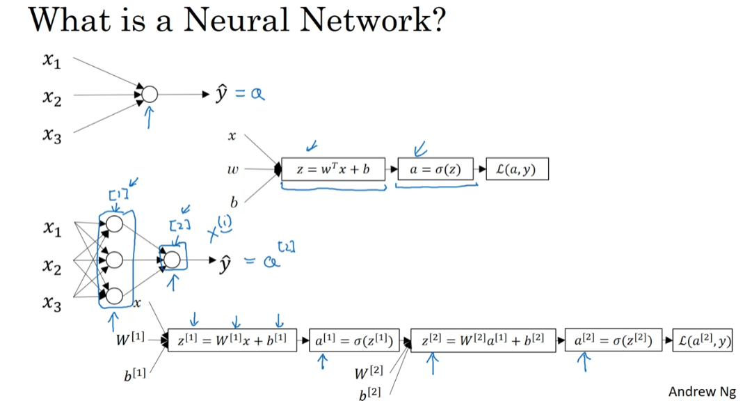
So, I know that was a lot of details but the key intuition to take away is that whereas for logistic regression, we had this z followed by a calculation. In this neural network, here we just do it multiple times, as a z followed by a calculation, and a z followed by a calculation, and then you finally compute the loss at the end.

You remember that for logistic regression, we had this backward calculation in order to compute derivatives or as you’re computing your d a, d z and so on. So, in the same way, a neural network will end up doing a backward calculation that looks like this in which you end up computing da_2, dz_2, that allows you to compute dw_2, db_2, and so on. This right to left backward calculation that is denoting with the red arrows.

So, that gives you a quick overview of what a neural network looks like. It’s basically taken logistic regression and repeating it twice. I know there was a lot of new notation laws, new details, don’t worry about saving them, follow everything, we’ll go into the details most probably in the next few videos. So, let’s go on to the next video. We’ll start to talk about the neural network representation.

Neural Network Representation

You see me draw a few
pictures of neural networks. In this video, we’ll talk about
exactly what those pictures means. In other words, exactly what those neural networks
that we’ve been drawing represent. And we’ll start with focusing on
the case of neural networks with what was called a single hidden layer.

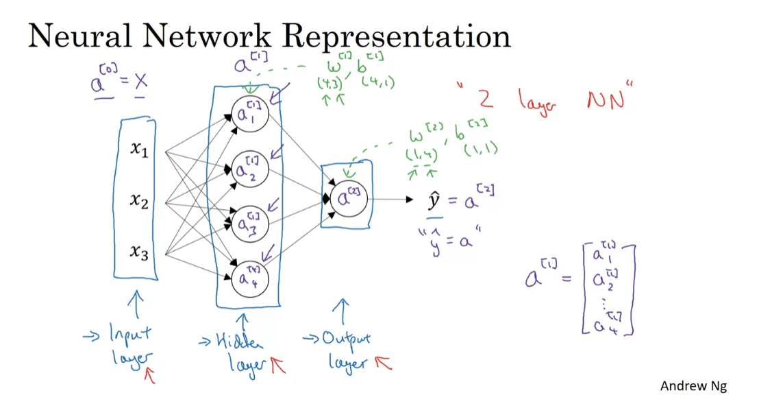
Here’s a picture of a neural network. Let’s give different parts of
these pictures some names. We have the input features, x1,
x2, x3 stacked up vertically. And this is called the input
layer of the neural network. So maybe not surprisingly, this contains
the inputs to the neural network. Then there’s another layer of circles. And this is called a hidden
layer of the neural network. I’ll come back in a second to
say what the word hidden means. But the final layer here is formed by,
in this case, just one node. And this single-node layer is called
the output layer, and is responsible for generating the predicted value y hat.

In a neural network that
you train with supervised learning, the training set contains values of the
inputs x as well as the target outputs y. So the term hidden layer refers to
the fact that in the training set, the true values for
these nodes in the middle are not observed. That is, you don’t see what they
should be in the training set. You see what the inputs are. You see what the output should be. But the things in the hidden layer
are not seen in the training set. So that kind of explains the name
hidden layer; just because you don’t see it in the training set.

Notation

Let’s introduce a bit more notation. Whereas previously, we were using the
vector X to denote the input features and alternative notation for the values of the input features will
be A superscript square bracket 0. And the term A also stands for
activations, and it refers to the values
that different layers of the neural network are passing
on to the subsequent layers. So the input layer passes on
the value x to the hidden layer, so we’re going to call that activations
of the input layer A super script 0.

hidden layer

The next layer, the hidden layer, will
in turn generate some set of activations, which I’m going to write as
A superscript square bracket 1. So in particular,
this first unit or this first node, we generate a value A superscript
square bracket 1 subscript 1. This second node we generate a value. Now we have a subscript 2 and so on. And so, A superscript square bracket 1, this is a four dimensional vector
you want in Python because the 4x1 matrix, or
a 4 column vector, which looks like this. And it’s four dimensional, because
in this case we have four nodes, or four units, or
four hidden units in this hidden layer.

output layer

And then finally,
the open layer regenerates some value A2, which is just a real number. And so
y hat is going to take on the value of A2. So this is analogous to how in
logistic regression we have y hat equals a and in logistic regression which we
only had that one output layer, so we don’t use the superscript
square brackets. But with our neural network,
we now going to use the superscript square bracket to explicitly indicate
which layer it came from. One funny thing about notational
conventions in neural networks is that this network that you’ve seen here
is called a two layer neural network. And the reason is that when we
count layers in neural networks, we don’t count the input layer. So the hidden layer is layer one and
the output layer is layer two.

In our notational convention, we’re
calling the input layer layer zero, so technically maybe there are three
layers in this neural network. Because there’s the input layer,
the hidden layer, and the output layer. But in conventional usage, if you
read research papers and elsewhere in the course, you see people refer to this
particular neural network as a two layer neural network, because we don’t count
the input layer as an official layer.

Finally, something that we’ll get to
later is that the hidden layer and the output layers will have
parameters associated with them. So the hidden layer will have
associated with it parameters w and b. And I’m going to write superscripts
square bracket 1 to indicate that these are parameters associated with
layer one with the hidden layer. We’ll see later that w will
be a 4 by 3 matrix and b will be a 4 by 1 vector in this example. Where the first coordinate four
comes from the fact that we have four nodes of our hidden units and
a layer, and three comes from the fact that
we have three input features. We’ll talk later about
the dimensions of these matrices. And it might make more sense at that time.

But in some of the output layers has
associated with it also, parameters w superscript square bracket 2 and
b superscript square bracket 2. And it turns out the dimensions
of these are 1 by 4 and 1 by 1. And these 1 by 4 is because the hidden
layer has four hidden units, the output layer has just one unit. But we will go over the dimension of these
matrices and vectors in a later video.

So you’ve just seen what a two
layered neural network looks like. That is a neural network
with one hidden layer. In the next video, let’s go deeper into exactly what
this neural network is computing. That is how this neural
network inputs x and goes all the way to
computing its output y hat.

Computing a Neural Network’s Output

In the last video, you saw what a single hidden layer neural network looks like. In this video, let’s go through the details of exactly how this neural network computes these outputs. What you see is that it is like logistic regression, but repeated a lot of times. Let’s take a look. So, this is how a two-layer neural network looks. Let’s go more deeply into exactly what this neural network computes. Now, we’ve said before that logistic regression, the circle in logistic regression, really represents two steps of computation rows. You compute z as follows, and a second, you compute the activation as a sigmoid function of z. So, a neural network just does this a lot more times. Let’s start by focusing on just one of the nodes in the hidden layer. Let’s look at the first node in the hidden layer. So, I’ve grayed out the other nodes for now.

So, similar to logistic regression on the left, this nodes in the hidden layer does two steps of computation. The first step and think of as the left half of this node, it computes z equals w transpose x plus b, and the notation we’ll use is, these are all quantities associated with the first hidden layer. So, that’s why we have a bunch of square brackets there. This is the first node in the hidden layer. So, that’s why we have the subscript one over there. So first, it does that, and then the second step, is it computes a_[1]1 equals sigmoid of z[1]_1, like so.

notational convention

So, for both z and a, the notational convention is that a, l, i, the l here in superscript square brackets, refers to the layer number, and the i subscript here, refers to the nodes in that layer. So, the node we’ll be looking at is layer one, that is a hidden layer node one. So, that’s why the superscripts and subscripts were both one, one. So, that little circle, that first node in the neural network, represents carrying out these two steps of computation.

Now, let’s look at the second node in the neural network, or the second node in the hidden layer of the neural network. Similar to the logistic regression unit on the left, this little circle represents two steps of computation. The first step is it computes z. This is still layer one, but now as a second node equals w transpose x, plus b_[1]2, and then a[1] two equals sigmoid of z_[1]_2. Again, feel free to pause the video if you want, but you can double-check that the superscript and subscript notation is consistent with what we have written here above in purple.

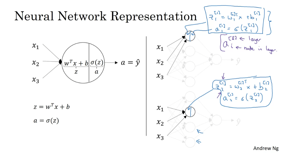
So, we’ve talked through the first two hidden units in a neural network, having units three and four also represents some computations. So now, let me take this pair of equations, and this pair of equations, and let’s copy them to the next slide. So, here’s our neural network, and here’s the first, and here’s the second equations that we’ve worked out previously for the first and the second hidden units. If you then go through and write out the corresponding equations for the third and fourth hidden units, you get the following. So, let me show this notation is clear, this is the vector w_[1]_1, this is a vector transpose times x. So, that’s what the superscript T there represents. It’s a vector transpose.

Now, as you might have guessed, if you’re actually implementing a neural network, doing this with a for loop, seems really inefficient. So, what we’re going to do, is take these four equations and vectorize. So, we’re going to start by showing how to compute z as a vector, it turns out you could do it as follows. Let me take these w’s and stack them into a matrix, then you have w_[1]1 transpose, so that’s a row vector, or this column vector transpose gives you a row vector, then w[1]2, transpose, w[1]3 transpose, w[1]4 transpose. So, by stacking those four w vectors together, you end up with a matrix. So, another way to think of this is that we have four logistic regression units there, and each of the logistic regression units, has a corresponding parameter vector, w. By stacking those four vectors together, you end up with this four by three matrix. So, if you then take this matrix and multiply it by your input features x1, x2, x3, you end up with by how matrix multiplication works. You end up with w[1]1 transpose x, w_2[1] transpose x, w_3_[1] transpose x, w_4_[1] transpose x. Then, let’s not figure the b’s. So, we now add to this a vector b_[1]1 one, b[1]2, b[1]3, b[1]4. So, that’s basically this, then this is b[1]1, b[1]2, b[1]3, b[1]4. So, you see that each of the four rows of this outcome correspond exactly to each of these four rows, each of these four quantities that we had above. So, in other words, we’ve just shown that this thing is therefore equal to z[1]1, z[1]2, z[1]3, z[1]4, as defined here. Maybe not surprisingly, we’re going to call this whole thing, the vector z[1], which is taken by stacking up these individuals of z’s into a column vector.

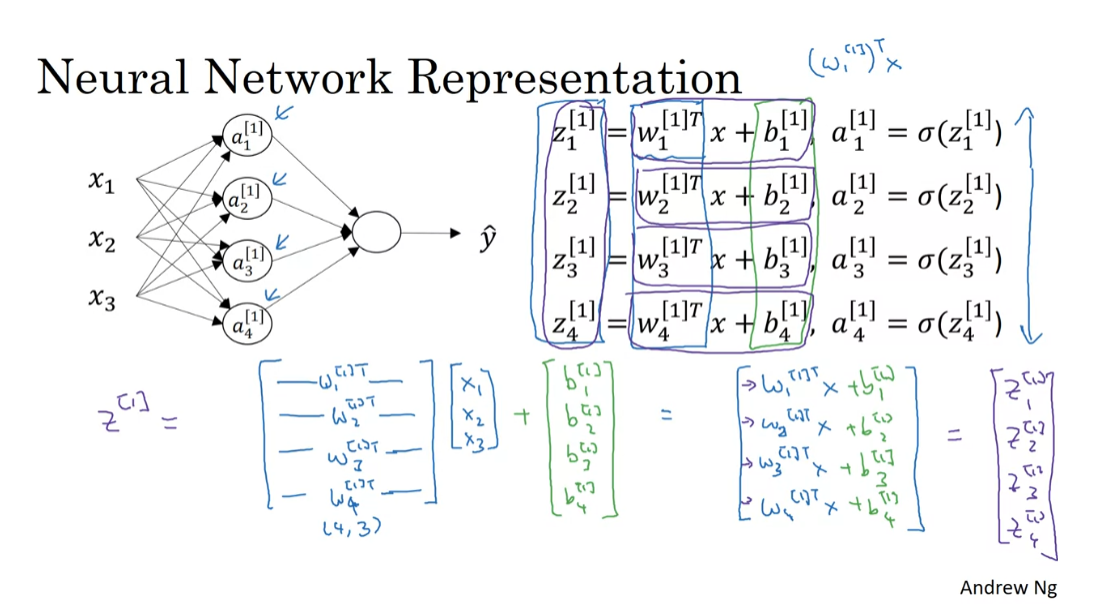
When we’re vectorizing, one of the rules of thumb that might help you navigate this, is that while we have different nodes in the layer, we’ll stack them vertically. So, that’s why we have z_[1]1 through z[1]4, those corresponded to four different nodes in the hidden layer, and so we stacked these four numbers vertically to form the vector z[1]. To use one more piece of notation, this four by three matrix here which we obtained by stacking the lowercase w[1]1, w[1]2, and so on, we’re going to call this matrix W capital [1]. Similarly, this vector, we’re going to call b superscript [1] square bracket. So, this is a four by one vector. So now, we’ve computed z using this vector matrix notation, the last thing we need to do is also compute these values of a. So, prior won’t surprise you to see that we’re going to define a[1], as just stacking together, those activation values, a [1], 1 through a [1], 4. So, just take these four values and stack them together in a vector called a[1]. This is going to be a sigmoid of z[1], where this now has been implementation of the sigmoid function that takes in the four elements of z, and applies the sigmoid function element-wise to it. _

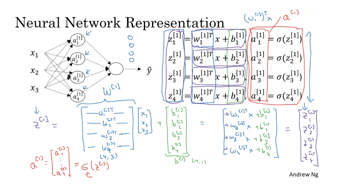
So, just a recap, we figured out that z_[1] is equal to w_[1] times the vector x plus the vector b_[1], and a_[1] is sigmoid times z_[1]. Let’s just copy this to the next slide. What we see is that for the first layer of the neural network given an input x, we have that z_[1] is equal to w_[1] times x plus b_[1], and a_[1] is sigmoid of z_[1]. The dimensions of this are four by one equals, this was a four by three matrix times a three by one vector plus a four by one vector b, and this is four by one same dimension as end. Remember, that we said x is equal to a_ [0]. Just say y hat is also equal to a two. If you want, you can actually take this x and replace it with a_[0], since a_[0] is if you want as an alias for the vector of input features, x. Now, through a similar derivation, you can figure out that the representation for the next layer can also be written similarly where what the output layer does is, it has associated with it, so the parameters w_[2] and b_[2]. So, w_[2] in this case is going to be a one by four matrix, and b_[2] is just a real number as one by on. So, z_[2] is going to be a real number we’ll write as a one by one matrix. Is going to be a one by four thing times a was four by one, plus b_[2] as one by one, so this gives you just a real number.

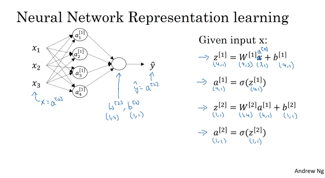
If you think of this last upper unit as just being analogous to logistic regression which have parameters w and b, w really plays an analogous role to w_[2] transpose, or w_[2] is really W transpose and b is equal to b_[2].

I said we want to cover up the left of this network and ignore all that for now, then this last upper unit is a lot like logistic regression, except that instead of writing the parameters as w and b, we’re writing them as w_[2] and b_[2], with dimensions one by four and one by one.

So, just a recap. For logistic regression, to implement the output or to implement prediction, you compute z equals w transpose x plus b, and a or y hat equals a, equals sigmoid of z. When you have a neural network with one hidden layer, what you need to implement, is to computer this output is just these four equations. You can think of this as a vectorized implementation of computing the output of first these for logistic regression units in the hidden layer, that’s what this does, and then this logistic regression in the output layer which is what this does.

I hope this description made sense, but the takeaway is to compute the output of this neural network, all you need is those four lines of code. So now, you’ve seen how given a single input feature, vector a, you can with four lines of code, compute the output of this neural network. Similar to what we did for logistic regression, we’ll also want to vectorize across multiple training examples. We’ll see that by stacking up training examples in different columns in the matrix, with just slight modification to this, you also, similar to what you saw in this regression, be able to compute the output of this neural network, not just a one example at a time, prolong your, say your entire training set at a time. So, let’s see the details of that in the next video.

Vectorizing Across Multiple Examples

In the last video, you saw how to compute
the prediction on a neural network, given a single training example. In this video, you see how to vectorize
across multiple training examples. And the outcome will be quite similar to
what you saw for logistic regression. Whereby stacking up different training
examples in different columns of the matrix, you’d be able to take the
equations you had from the previous video. And with very little modification, change
them to make the neural network compute the outputs on all the examples on
pretty much all at the same time.

So let’s see the details
on how to do that. These were the four equations we have from
the previous video of how you compute z1, a1, z2 and a2. And they tell you how,
given an input feature back to x, you can use them to generate a2 =y hat for
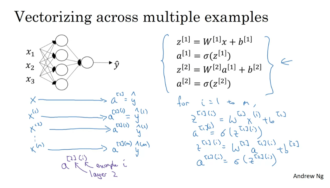
a single training example. Now if you have m training examples,
you need to repeat this process for say, the first training example. x superscript (1) to compute y hat 1 does a prediction on
your first training example. Then x(2) use that to generate
prediction y hat (2). And so on down to x(m) to
generate a prediction y hat (m). And so in all these activation
function notation as well, I’m going to write this as a2. And this is a2, and a(2)(m), so this notation a2. The round bracket i refers
to training example i, and the square bracket 2
refers to layer 2, okay.

So that’s how the square bracket and
the round bracket indices work. And so to suggest that if you have
an unvectorized implementation and want to compute the predictions
of all your training examples, you need to do for i = 1 to m. Then basically implement
these four equations, right? You need to make a z1 = W(1) x(i) + b[1], a1 = sigma of z1. z2 = w[2]a1 + b[2] andZ2i equals w2a1i plus b2 and a2 = sigma point of z2. So it’s basically these four equations
on top by adding the superscript round bracket i to all the variables that
depend on the training example. So adding this superscript round
bracket i to x is z and a, if you want to compute all the outputs
on your m training examples examples.

What we like to do is vectorize this whole
computation, so as to get rid of this for. And by the way, in case it seems like
I’m getting a lot of nitty gritty linear algebra, it turns out that
being able to implement this correctly is important in
the deep learning era. And we actually chose notation
very carefully for this course and make this vectorization
steps as easy as possible. So I hope that going through this
nitty gritty will actually help you to more quickly get correct implementations
of these algorithms working.

Alright, so let me just copy this whole
block of code to the next slide and then we’ll see how to vectorize this. So here’s what we have from
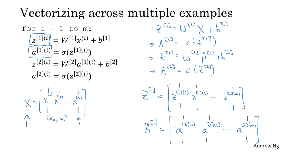
the previous slide with the for loop going over our m training examples. So recall that we defined
the matrix x to be equal to our training examples stacked
up in these columns like so. So take the training examples and
stack them in columns. So this becomes a n, or maybe nx by m diminish the matrix. I’m just going to give away the punch line
and tell you what you need to implement in order to have a vectorized
implementation of this for loop. It turns out what you
need to do is compute Z[1] = W[1] X + b[1], A[1]= sig point of z[1]. Then Z[2] = w[2] A[1] + b[2] and then A[2] = sig point of Z[2].

So if you want the analogy is that
we went from lower case vector xs to just capital case X matrix by stacking
up the lower case xs in different columns. If you do the same thing for
the zs, so for example, if you take z1, z1, and so on, and these are all column vectors,
up to z1, right. So that’s this first quantity that all
m of them, and stack them in columns. Then just gives you the matrix z[1]. And similarly you look
at say this quantity and take a1, a1 and so on and a1, and stacked them up in columns. Then this, just as we went from
lower case x to capital case X, and lower case z to capital case Z. This goes from the lower case a,
which are vectors to this capital A[1], that’s over there and
similarly, for z[2] and a[2]. Right they’re also obtained
by taking these vectors and stacking them horizontally. And taking these vectors and
stacking them horizontally, in order to get Z[2], and E[2].

One of the property of this
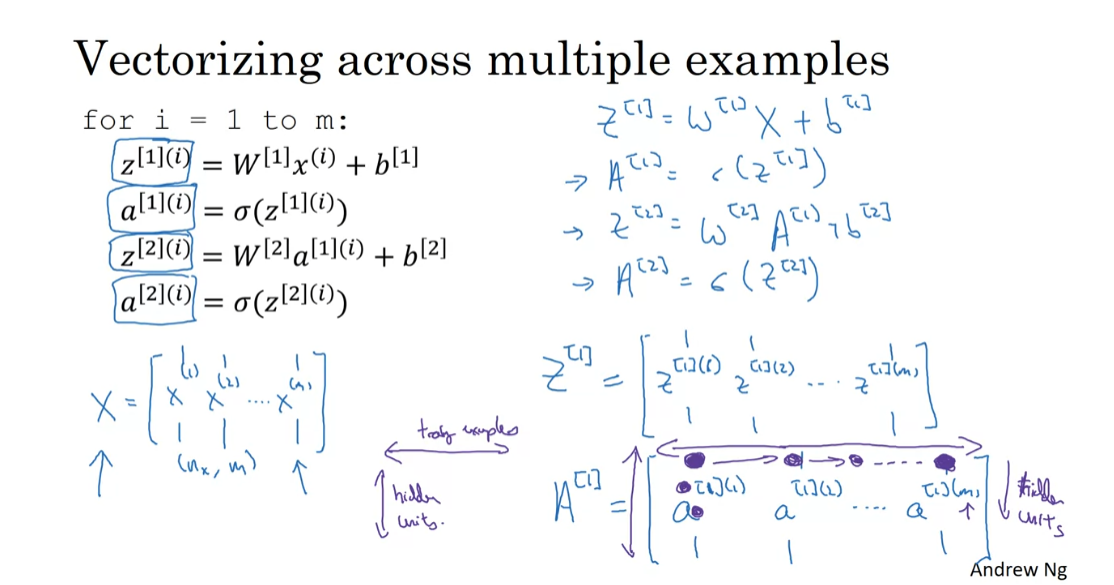
notation that might help you to think about it is that
this matrixes say Z and A, horizontally we’re going to
index across training examples. So that’s why the horizontal index
corresponds to different training example, when you sweep from left to right you’re
scanning through the training cells. And vertically this vertical index
corresponds to different nodes in the neural network. So for example, this node,
this value at the top most, top left most corner of the mean
corresponds to the activation of the first heading unit on
the first training example. One value down corresponds to the
activation in the second hidden unit on the first training example, then the third heading unit on
the first training sample and so on. So as you scan down this is your
indexing to the hidden units number.

Whereas if you move horizontally, then
you’re going from the first hidden unit. And the first training example
to now the first hidden unit and the second training sample,
the third training example. And so on until this node here corresponds
to the activation of the first hidden unit on the final train example and
the nth training example. Okay so the horizontally the matrix
A goes over different training examples. And vertically the different
indices in the matrix A corresponds to different hidden units. And a similar intuition holds true for
the matrix Z as well as for X where horizontally corresponds
to different training examples. And vertically it corresponds to
different input features which are really different than those of
the input layer of the neural network. So of these equations, you now know
how to implement in your network with vectorization, that is
vectorization across multiple examples. In the next video I want to show you
a bit more justification about why this is a correct implementation
of this type of vectorization. It turns out the justification would be
similar to what you had seen in logistic regression. Let’s go on to the next video.

Explanation for Vectorized Implementation

In the previous video, we saw how with your training examples stacked up horizontally in the matrix x, you can derive a vectorized implementation for propagation through your neural network. Let’s give a bit more justification for why the equations we wrote down is a correct implementation of vectorizing across multiple examples.

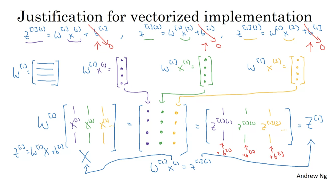
So let’s go through part of the forward propagation calculation for the few examples. Let’s say that for the first training example, you end up computing this x1 plus b1 and then for the second training example, you end up computing this x2 plus b1 and then for the third training example, you end up computing this 3 plus b1. So, just to simplify the explanation on this slide, I’m going to ignore b. So let’s just say, to simplify this justification a little bit that b is equal to zero. But the argument we’re going to lay out will work with just a little bit of a change even when b is non-zero. It does just simplify the description on the slide a bit. Now, w1 is going to be some matrix, right? So I have some number of rows in this matrix. So if you look at this calculation x1, what you have is that w1 times x1 gives you some column vector which you must draw like this. And similarly, if you look at this vector x2, you have that w1 times x2 gives some other column vector, right? And that’s gives you this z12. And finally, if you look at x3, you have w1 times x3, gives you some third column vector, that’s this z13.

So now, if you consider the training set capital X, which we form by stacking together all of our training examples. So the matrix capital X is formed by taking the vector x1 and stacking it vertically with x2 and then also x3. This is if we have only three training examples. If you have more, you know, they’ll keep stacking horizontally like that. But if you now take this matrix x and multiply it by w then you end up with, if you think about how matrix multiplication works, you end up with the first column being these same values that I had drawn up there in purple. The second column will be those same four values. And the third column will be those orange values, what they turn out to be. But of course this is just equal to z11 expressed as a column vector followed by z12 expressed as a column vector followed by z13, also expressed as a column vector. And this is if you have three training examples. You get more examples then there’d be more columns. And so, this is just our matrix capital Z1.

So I hope this gives a justification for why we had previously w1 times xi equals z1i when we’re looking at single training example at the time. When you took the different training examples and stacked them up in different columns, then the corresponding result is that you end up with the z’s also stacked at the columns. And I won’t show but you can convince yourself if you want that with Python broadcasting, if you add back in, these values of b to the values are still correct. And what actually ends up happening is you end up with Python broadcasting, you end up having bi individually to each of the columns of this matrix. So on this slide, I’ve only justified that z1 equals w1x plus b1 is a correct vectorization of the first step of the four steps we have in the previous slide, but it turns out that a similar analysis allows you to show that the other steps also work on using a very similar logic where if you stack the inputs in columns then after the equation, you get the corresponding outputs also stacked up in columns.

Finally, let’s just recap everything we talked about in this video. If this is your neural network, we said that this is what you need to do if you were to implement for propagation, one training example at a time going from i equals 1 through m. And then we said, let’s stack up the training examples in columns like so and for each of these values z1, a1, z2, a2, let’s stack up the corresponding columns as follows. So this is an example for a1 but this is true for z1, a1, z2, and a2. Then what we show on the previous slide was that this line allows you to vectorize this across all m examples at the same time. And it turns out with the similar reasoning, you can show that all of the other lines are correct vectorizations of all four of these lines of code.

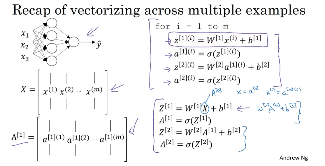
And just as a reminder, because x is also equal to a0 because remember that the input feature vector x was equal to a0, so xi equals a0i. Then there’s actually a certain symmetry to these equations where this first equation can also be written z1 = w1 a0 + b1. And so, you see that this pair of equations and this pair of equations actually look very similar but just of all of the indices advance by one. So this kind of shows that the different layers of a neural network are roughly doing the same thing or just doing the same computation over and over. And here we have two-layer neural network where we go to a much deeper neural network in next week’s videos. You see that even deeper neural networks are basically taking these two steps and just doing them even more times than you’re seeing here.

So that’s how you can vectorize your neural network across multiple training examples. Next, we’ve so far been using the sigmoid functions throughout our neural networks. It turns out that’s actually not the best choice. In the next video, let’s dive a little bit further into how you can use different, what’s called, activation functions of which the sigmoid function is just one possible choice.

Activation Functions

When you build your neural network,
one of the choices you get to make is what activation function to
use in the hidden layers as well as at the output
units of your neural network. So far, we’ve just been using
the sigmoid activation function, but sometimes other choices
can work much better. Let’s take a look at some of the options. In the forward propagation steps for
the neural network, we had these two steps where we
use the sigmoid function here. So that sigmoid is called
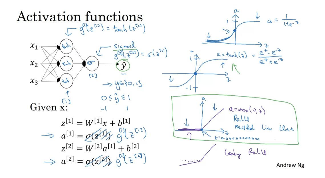
an activation function. And here’s the familiar sigmoid function, a = 1/(1 + e to -z). So in the more general case, we can have a different function g(z). Which I’m going to write here where
g could be a nonlinear function that may not be the sigmoid function.

So for example, the sigmoid
function goes between zero and one. An activation function that almost
always works better than the sigmoid function is the tangent function or
the hyperbolic tangent function. So this is z, this is a,
this is a = tan h(z). And this goes between +1 and -1. The formula for the tan h function is e to the z minus e to-z over their sum. And it’s actually mathematically a shifted
version of the sigmoid function. So as a sigmoid function just
like that but shifted so that it now crosses the zero
zero point on the scale. So it goes between minus one and plus one.

And it turns out that for hidden units, if you let the function
g(z) be equal to tan h(z). This almost always works better than
the sigmoid function because with values between plus one and minus one,
the mean of the activations that come out of your hidden layer are closer
to having a zero mean. And so just as sometimes when
you train a learning algorithm, you might center the data and have your data have zero mean using
a tan h instead of a sigmoid function. Kind of has the effect of
centering your data so that the mean of your data is close
to zero rather than maybe 0.5. And this actually makes learning for
the next layer a little bit easier.

We’ll say more about this in the second
course when we talk about optimization algorithms as well. But one takeaway is that
I pretty much never use the sigmoid activation function anymore. The tan h function is almost
always strictly superior. The one exception is for the output
layer because if y is either zero or one, then it makes sense for
y hat to be a number that you want to output that’s between zero and
one rather than between -1 and 1. So the one exception where I would use
the sigmoid activation function is when you’re using binary classification. In which case you might use the sigmoid
activation function for the upper layer. So g(z2) here is equal to sigmoid of z2.

And so what you see in this
example is where you might have a tan h activation function for the hidden
layer and sigmoid for the output layer. So the activation functions can be
different for different layers. And sometimes to denote that
the activation functions are different for different layers, we might use these square brackets
superscripts as well to indicate that gf square bracket one may be different
than gf square bracket two, right. Again, square bracket one
superscript refers to this layer and superscript square bracket two
refers to the output layer.

Now, one of the downsides of
both the sigmoid function and the tan h function is that if z is
either very large or very small, then the gradient of the derivative of the
slope of this function becomes very small. So if z is very large or z is very small,
the slope of the function either ends up being close to zero and so
this can slow down gradient descent. So one other choice that is very
popular in machine learning is what’s called the rectified linear unit. So the RELU function looks like this and the formula is a = max(0,z). So the derivative is one so
long as z is positive and derivative or
the slope is zero when z is negative.

If you’re implementing this, technically the derivative when z is
exactly zero is not well defined. But when you implement
this in the computer, the odds that you get exactly z
equals 000000000000 is very small. So you don’t need to worry about it. In practice, you could pretend
a derivative when z is equal to zero, you can pretend is either one or zero. And you can work just fine. So the fact is not differentiable.

The fact that, so here’s some rules of
thumb for choosing activation functions. If your output is zero one value,
if you’re using binary classification, then the sigmoid activation function is
very natural choice for the output layer. And then for all other units relu or the rectified linear unit is increasingly the default choice of activation function. So if you’re not sure what to use for
your hidden layer, I would just use the relu activation function, is what
you see most people using these days. Although sometimes people also use
the tan h activation function.

One disadvantage of the value is that
the derivative is equal to zero when z is negative. In practice this works just fine. But there is another version of
the value called the Leaky ReLU. We’ll give you the formula on the next
slide but instead of it being zero when z is negative,
it just takes a slight slope like so. So this is called Leaky ReLU. This usually works better than
the value activation function. Although, it’s just not
used as much in practice. Either one should be fine. Although, if you had to pick one,
I usually just use the relu. And the advantage of both the value and
the Leaky ReLU is that for a lot of the space of z,
the derivative of the activation function, the slope of the activation function
is very different from zero. And so in practice,
using the value activation function, your neural network will often learn
much faster than when using the tan h or the sigmoid activation function. And the main reason is that there’s
less of this effect of the slope of the function going to zero,
which slows down learning. And I know that for half of the range
of z, the slope for value is zero. But in practice, enough of your hidden
units will have z greater than zero. So learning can still be quite fast for
most training examples.

Pros and cons

So let’s just quickly recap the pros and
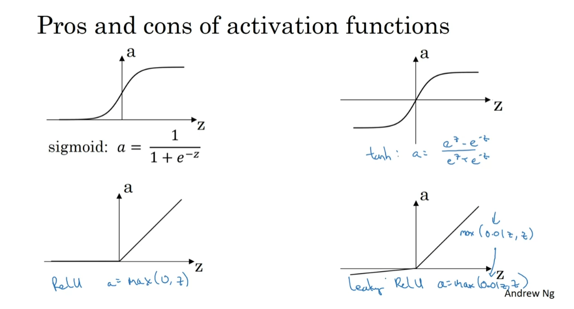
cons of different activation functions. Here’s the sigmoid activation function. I would say never use this except for
the output layer if you’re doing binomial classification or
maybe almost never use this. And the reason I almost never
use this is because the tan h is pretty much strictly superior. So the tan h activation function is this. And then the default, the most commonly used activation
function is the ReLU, which is this. So if you’re not sure what else to use,
use this one. And maybe, feel free also to try the Leaky ReLU where might be 0.01(z,z), right? So a is the max of 0.1 times z and z. So that gives you this
bend in the function. And you might say,
why is that constant 0.01? Well, you can also make that another
parameter of the learning algorithm. And some people say that works even
better, but how they see people do that.

So, but if you feel like trying it in your
application, please feel free to do so. And you can just see how it works and
how well it works, and stick with it if it
gives you a good result.

So I hope that gives you a sense of some
of the choices of activation functions you can use in your neural network. One of the things we’ll see in deep
learning is that you often have a lot of different choices in how you
build your neural network. Ranging from a number of hidden units
to the choices activation function, to how you initialize the ways
which we’ll see later. A lot of choices like that. And it turns out that it is sometimes
difficult to get good guidelines for exactly what will work best for
your problem.

So throughout these courses,
I’ll keep on giving you a sense of what I see in the industry in terms of
what’s more or less popular. But for your application with your
applications, idiosyncrasies is actually very difficult to know in advance
exactly what will work best. So common piece of advice would be,
if you’re not sure which one of these activation functions work best,
try them all. And evaluate on like a holdout validation
set or like a development set, which we’ll talk about later. And see which one works better and
then go of that. And I think that by testing
these different choices for your application, you’d be better
at future proofing your neural network architecture against
the idiosyncracies problems. As well as evolutions of
the algorithms rather than, if I were to tell you always use a ReLU
activation and don’t use anything else. That just may or may not apply for
whatever problem you end up working on. Either in the near future or
in the distant future.

All right, so, that was choice
of activation functions and you see the most popular
activation functions. There’s one other question that
sometimes you can ask which is, why do you even need to use
an activation function at all? Why not just do away with that? So, let’s talk about that in the next
video where you see why neural networks do need some sort of
non linear activation function.

Why do you need Non-Linear Activation Functions?

Why does a neural network need
a non-linear activation function? Turns out that your neural network
to compute interesting functions, you do need to pick a non-linear
activation function, let’s see one. So, here’s the four prop equations for
the neural network. Why don’t we just get rid of this? Get rid of the function g? And set a1 equals z1. Or alternatively, you can say that
g of z is equal to z, all right? Sometimes this is called
the linear activation function. Maybe a better name for it would be
the identity activation function because it just outputs
whatever was input. For the purpose of this,
what if a(2) was just equal z(2)? It turns out if you do this,
then this model is just computing y or y-hat as a linear function
of your input features, x, to take the first two equations. If you have that a(1) = Z(1) = W(1)x + b, and then a(2) = z (2) = W(2)a(1) + b. Then if you take this definition of a1 and plug it in there, you find that a2 = w2(w1x + b1), move that up a bit. Right?
So this is a1 + b2, and so this simplifies to: (W2w1)x + (w2b1 + b2). So this is just, let’s call this w prime b prime.

So this is just equal to w’ x + b’. If you were to use linear
activation functions or we can also call them identity
activation functions, then the neural network is just outputting
a linear function of the input. And we’ll talk about deep networks later,
neural networks with many, many layers, many hidden layers. And it turns out that if you use a linear activation function or
alternatively, if you don’t have an activation function,
then no matter how many layers your neural network has, all it’s doing is just
computing a linear activation function.

So you might as well not
have any hidden layers. Some of the cases that are briefly
mentioned, it turns out that if you have a linear activation function here and a
sigmoid function here, then this model is no more expressive than standard logistic
regression without any hidden layer. So I won’t bother to prove that, but
you could try to do so if you want. But the take home is that a linear
hidden layer is more or less useless because the composition of two linear
functions is itself a linear function.

So unless you throw a non-linear item
in there, then you’re not computing more interesting functions even as you
go deeper in the network. There is just one place where you might
use a linear activation function. g(x) = z. And that’s if you are doing machine
learning on the regression problem. So if y is a real number. So for example, if you’re trying
to predict housing prices. So y is not 0, 1, but is a real
number, anywhere from - I don’t know - $0 is the price of house up to however
expensive, right, houses get, I guess. Maybe houses can be potentially
millions of dollars, so however much houses cost in your data set.

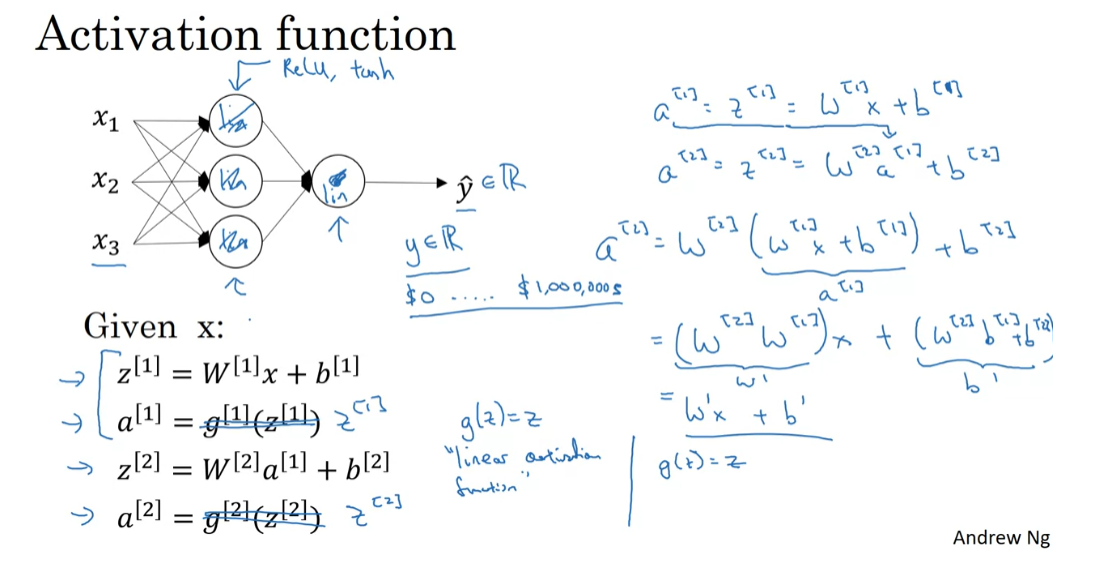
But if y takes on these real values, then it might be okay to have
a linear activation function here so that your output y hat is also a real number going anywhere from
minus infinity to plus infinity. But then the hidden units should
not use the activation functions. They could use ReLU or tanh or
Leaky ReLU or maybe something else. So the one place you might use
a linear activation function is usually in the output layer.

But other than that, using a linear
activation function in the hidden layer except for some very special circumstances
relating to compression that we’re going to talk about using the linear
activation function is extremely rare. And, of course, if we’re
actually predicting housing prices, as you saw in the week one video, because
housing prices are all non-negative, Perhaps even then you can use
a value activation function so that your output y-hats are all
greater than or equal to 0.

So I hope that gives you a sense of
why having a non-linear activation function is a critical
part of neural networks. Next we’re going to start to
talk about gradient descent and to do that to set up for
our discussion for gradient descent, in the next video I want to show you how
to estimate-how to compute-the slope or the derivatives of individual
activation functions. So let’s go on to the next video.

激活函数在神经网络中起着至关重要的作用，主要有以下几个原因：

1. 引入非线性特性： 激活函数引入了非线性特性，使神经网络可以学习和表示更复杂的函数关系。如果没有激活函数，多层神经网络就会退化成一个简单的线性模型，无法捕捉到非线性模式。

2. 使神经网络逼近任意函数： 通过使用适当的激活函数，神经网络可以逼近任意复杂的函数，这是基于 universality theorem 的结果。

3. 梯度传播： 激活函数对于梯度的传播至关重要。在反向传播算法中，通过梯度计算来更新网络参数。激活函数的导数决定了梯度的传播方式，从而影响网络的学习速度和稳定性。

4. 限制输出范围： 某些激活函数可以将神经元的输出限制在特定的范围内，比如 [0, 1] 或 [-1, 1]，这有助于防止梯度爆炸或梯度消失的问题。

综上所述，激活函数在神经网络中是不可或缺的，它们使神经网络能够学习和逼近复杂的非线性函数，并且在训练过程中起到关键的作用。

Derivatives of Activation Functions

When you implement back propagation
for your neural network, you need to either compute the slope or
the derivative of the activation functions. So, let’s take a look at our choices of activation functions and how you can
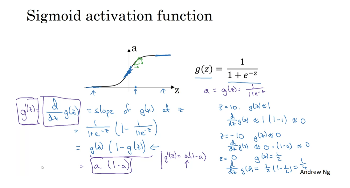
compute the slope of these functions. Here’s the familiar Sigmoid
activation function. So, for any given value of z, maybe this value of z. This function will have some slope or
some derivative corresponding to, if you draw a little line there, the height over width of this
lower triangle here. So, if g of z is the sigmoid function, then the slope of the function is d, dz g of z, and so we know from calculus that
it is the slope of g of x at z. If you are familiar with calculus
and know how to take derivatives, if you take the derivative of
the Sigmoid function, it is possible to show that it is
equal to this formula. Again, I’m not going to do
the calculus steps, but if you are familiar with calculus, feel free to pause a video and
try to prove this yourself. So, this is equal to just g of z, times 1 minus g of z.

So, let’s just sanity check that
this expression make sense. First, if z is very large, so say z is equal to 10, then g of z will be close to 1, and so the formula we have on the left tells
us that d dz g of z does be close to g of z, which is equal to 1 times 1 minus 1, which is therefore very close to 0. This isn’t the correct because
when z is very large, the slope is close to 0. Conversely, if z is equal to minus 10, so it says well there, then g of z is close to 0. So, the formula on the left tells us
d dz g of z would be close to g of z, which is 0 times 1 minus 0. So it is also very close to 0,
which is correct. Finally, if z is equal to 0, then g of z is equal to one-half, that’s the sigmoid function right here, and so the derivative is equal to
one-half times 1 minus one-half, which is equal to one-quarter, and that actually turns out to
be the correct value of the derivative or the slope of this
function when z is equal to 0.

Finally, just to introduce
one more piece of notation, sometimes instead of writing this thing, the shorthand for the derivative
is g prime of z. So, g prime of z in calculus, the little dash on top is called prime, but so g prime of z is a
shorthand for the calculus for the derivative of the function of g
with respect to the input variable z. Then in a neural network, we have a equals g of z, equals this, then this formula
also simplifies to a times 1 minus a.

So, sometimes in implem entation, you might see something like
g prime of z equals a times 1 minus a, and that just refers to the
observation that g prime, which just means the derivative, is equal to this over here. The advantage of this formula is that
if you’ve already computed the value for a, then by using this expression, you can very quickly compute the
value for the slope for g prime as well. All right. So, that was the
sigmoid activation function.

Let’s now look at the Tanh
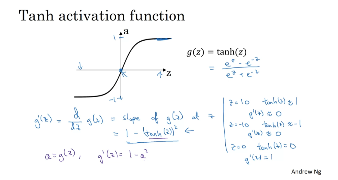
activation function. Similar to what we had previously, the definition of d dz g of z is the slope of g of z at
a particular point of z, and if you look at the formula for
the hyperbolic tangent function, and if you know calculus, you can take derivatives and
show that this simplifies to this formula and using the shorthand we have previously
when we call this g prime of z again. So, if you want you can sanity check
that this formula makes sense.

So, for example, if z is equal to 10, Tanh of z will be very close to 1. This goes from plus 1 to minus 1. Then g prime of z, according to this formula, would be about 1 minus 1 squared, so there’s very close to 0. So, that was if z is very large, the slope is close to 0. Conversely, if z is very small, say z is equal to minus 10, then Tanh of z will be close to minus 1, and so g prime of z will be
close to 1 minus negative 1 squared. So, it’s close to 1 minus 1, which is also close to 0. Then finally, if z is equal to 0, then Tanh of z is equal to 0, and then the slope is
actually equal to 1, which is actually the slope
when z is equal to 0.

So, just to summarize, if a is equal to g of z, so if a is equal to this
Tanh of z, then the derivative, g prime of z, is equal to
1 minus a squared. So, once again, if you’ve already
computed the value of a, you can use this formula to very
quickly compute the derivative as well.

Finally, here’s how you
compute the derivatives for the ReLU and Leaky ReLU
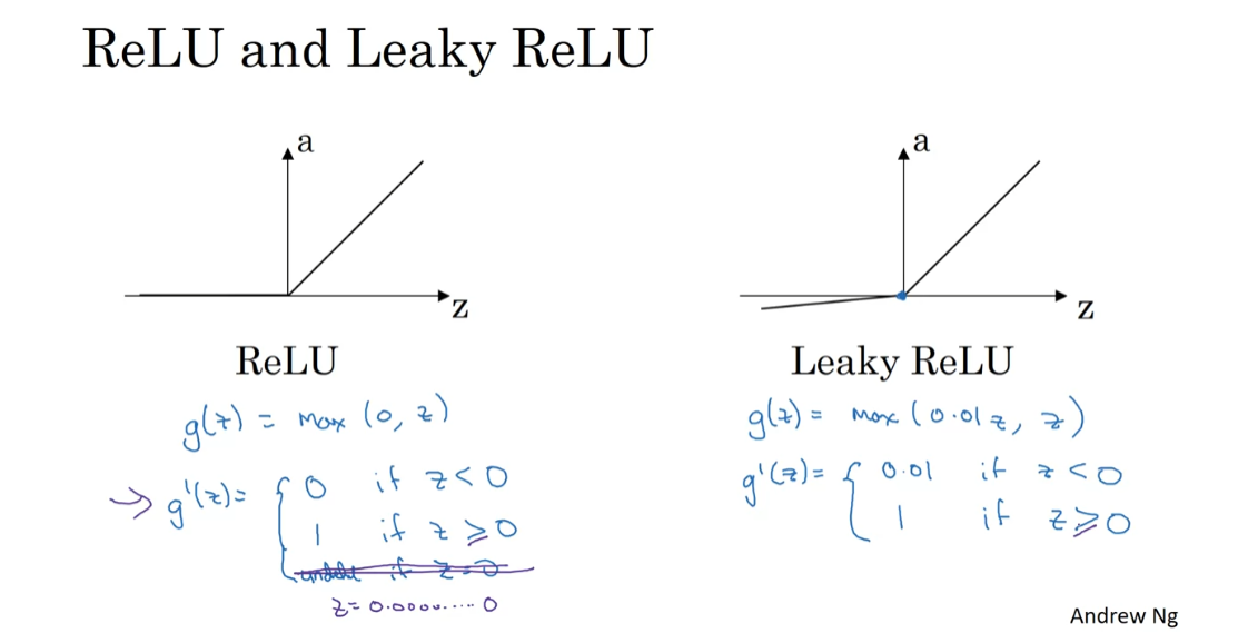
activation functions. For the value g of z is
equal to max of 0,z, so the derivative is equal to, turns out to be 0 , if z is less than 0 and 1
if z is greater than 0. It’s actually undefined, technically
undefined if z is equal to exactly 0. But if you’re implementing
this in software, it might not be a 100 percent
mathematically correct, but it’ll work just fine
if z is exactly a 0, if you set the derivative
to be equal to 1. It always had to be 0,
it doesn’t matter. If you’re an expert in
optimization, technically, g prime then becomes what’s called a
sub-gradient of the activation function g of z, which is why gradient
descent still works. But you can think of it as that, the chance of z being
exactly 0.000000. It’s so small that it almost
doesn’t matter where you set the derivative to be equal to
when z is equal to 0. So, in practice, this is what
people implement for the derivative of z.

Finally, if you are training a neural network
with a Leaky ReLU activation function, then g of z is going to be
max of say 0.01 z, z, and so, g prime of z is equal to 0.01 if z is less than 0 and 1 if z is greater than 0. Once again, the gradient is technically
not defined when z is exactly equal to 0, but if you implement a
piece of code that sets the derivative or that sets
g prime to either 0.01 or or to 1, either way, it doesn’t really matter. When z is exactly 0,
your code will work just. So, under these formulas, you should either compute the slopes or
the derivatives of your activation functions. Now that we have this building block, you’re ready to see how to implement
gradient descent for your neural network. Let’s go on to the next video to see that.

Gradient Descent for Neural Networks

All right. I think this’ll be an exciting video. In this video, you’ll see how to implement gradient descent for your neural network
with one hidden layer. In this video, I’m going to just give you
the equations you need to implement in order to get back-propagation
or to get gradient descent working, and then in the video after this one, I’ll give some more intuition about why these particular equations are the
accurate equations, are the correct equations for computing the
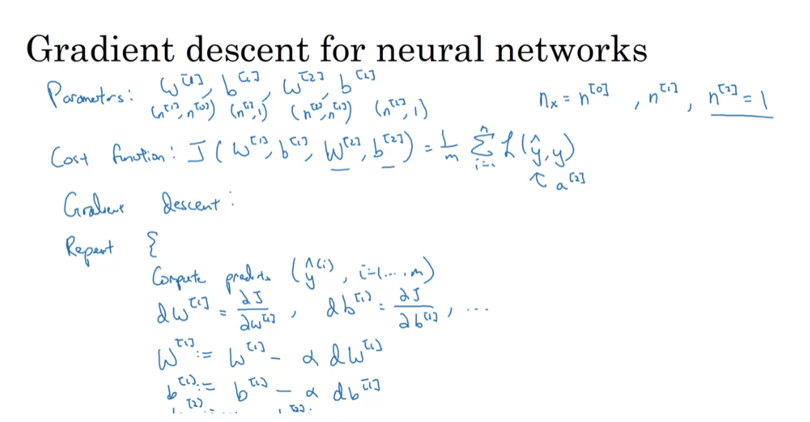
gradients you need for your neural network. So, your neural network, with a single hidden layer for now, will have parameters W1, B1, W2, and B2. So, as a reminder, if you have NX or alternatively N0 input features, and N1 hidden units, and N2 output units in our examples. So far I’ve only had N2 equals one, then the matrix W1 will be N1 by N0. B1 will be an N1 dimensional vector, so we can write that as N1
by one-dimensional matrix, really a column vector. The dimensions of W2 will be N2 by N1, and the dimension of B2 will be N2 by one. Right, so far we’ve only
seen examples where N2 is equal to one, where you have just one single hidden unit. So, you also have a cost function
for a neural network. For now, I’m just going to assume
that you’re doing binary classification. So, in that case, the cost of your parameters as
follows is going to be one over M of the average of that loss function. So, L here is the loss when your
neural network predicts Y hat, right. This is really A2 when the
gradient label is equal to Y. If you’re doing binary classification, the loss function can be exactly what
you use for logistic regression earlier. So, to train the parameters of your algorithm, you need to perform gradient descent. When training a neural network, it is important to initialize the parameters
randomly rather than to all zeros. We’ll see later why that’s the case, but after initializing the parameter
to something, each loop or gradient descents
with computed predictions. So, you basically compute your Y hat I, for I equals one through M, say. Then, you need to compute the derivative. So, you need to compute DW1, and that’s the derivative of the cost function
with respect to the parameter W1, you can compute another variable, shall I call DB1, which is the derivative or the slope
of your cost function with respect to the variable B1 and so on. Similarly for the other parameters W2 and B2. Then finally, the gradient descent update
would be to update W1 as W1 minus Alpha. The learning rate times D, W1. B1 gets updated as B1 minus the learning rate, times DB1, and similarly for W2 and B2. Sometimes, I use colon equals
and sometimes equals, as either notation works fine. So, this would be one iteration
of gradient descent, and then you repeat this some number of times until your parameters
look like they’re converging.

So, in previous videos, we talked about how to
compute the predictions, how to compute the outputs, and we saw how to do that in
a vectorized way as well. So, the key is to know how to compute
these partial derivative terms, the DW1, DB1 as well as the
derivatives DW2 and DB2. So, what I’d like to do is just give you the equations you need in order to
compute these derivatives. I’ll defer to the next video, which
is an optional video, to go greater into Jeff about how we
came up with those formulas. So, let me just summarize again
the equations for propagation. So, you have Z1 equals W1X plus B1, and then A1 equals the activation function
in that layer applied element wise as Z1, and then Z2 equals W2, A1 plus V2, and then finally, just as all vectorized across your training set, right? A2 is equal to G2 of Z2. Again, for now, if we assume we’re
doing binary classification, then this activation function really
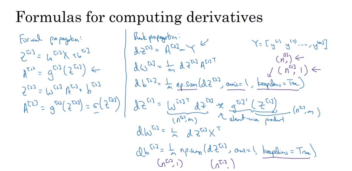
should be the sigmoid function, same just for that end neural. So, that’s the forward propagation or the left to right for computation for your neural network. Next, let’s compute the derivatives. So, this is the back propagation step. Then I compute DZ2 equals A2
minus the gradient of Y, and just as a reminder, all this is vectorized across examples. So, the matrix Y is this one by M matrix that lists all of your M
examples stacked horizontally. Then it turns out DW2 is equal to this, and in fact, these first three equations are very similar to gradient descents
for logistic regression. X is equals one, comma, keep dims equals true. Just a little detail this np.sum is a Python NumPy command for summing
across one-dimension of a matrix. In this case, summing horizontally, and what keepdims does is,
it prevents Python from outputting one of those funny
rank one arrays, right? Where the dimensions was your N comma. So, by having keepdims equals true, this ensures that Python outputs for
DB a vector that is N by one. In fact, technically this will be I guess N2 by one. In this case, it’s just a one by one number, so maybe it doesn’t matter. But later on, we’ll see when it really matters.

So, so far what we’ve done is very
similar to logistic regression. But now as you continue to
run back propagation, you will compute this, DZ2 times G1 prime of Z1. So, this quantity G1 prime is the derivative of whether it was the activation
function you use for the hidden layer, and for the output layer, I assume that you are doing binary
classification with the sigmoid function. So, that’s already baked
into that formula for DZ2, and his times is element-wise product. So, this here is going to be an N1
by M matrix, and this here, this element-wise derivative thing is
also going to be an N1 by N matrix, and so this times there is an element-wise
product of two matrices. Then finally, DW1 is equal to that, and DB1 is equal to this, and p.sum DZ1 axis equals one, keepdims equals true. So, whereas previously the keepdims
maybe matter less if N2 is equal to one. Result is just a one by one
thing, is just a real number. Here, DB1 will be a N1 by one vector, and so you want Python, you want Np.sons. I’ll put something of this dimension rather
than a funny rank one array of that dimension which could end up
messing up some of your data calculations. The other way would be to not
have to keep the parameters, but to explicitly reshape the
output of NP.sum into this dimension, which you would like DB to have.

So, that was forward propagation
in I guess four equations, and back-propagation in I guess six equations. I know I just wrote down these equations, but in the next optional video, let’s go over some intuitions for how the six equations for the back
propagation algorithm were derived. Please feel free to watch that or not. But either way, if you
implement these algorithms, you will have a correct implementation
of forward prop and back prop. You’ll be able to compute the derivatives
you need in order to apply gradient descent, to learn the parameters of your neural network. It is possible to implement this algorithm and get it to work without deeply
understanding the calculus. A lot of successful deep
learning practitioners do so. But, if you want, you can also watch the next video, just to get a bit more intuition of
what the derivation of these equations.

Backpropagation Intuition (Optional)

In the last video, you saw the equations for
back-propagation. In this video, let’s go
over some intuition using the computation graph for how those equations
were derived. This video is
completely optional so feel free to watch it or not. You should be able to do
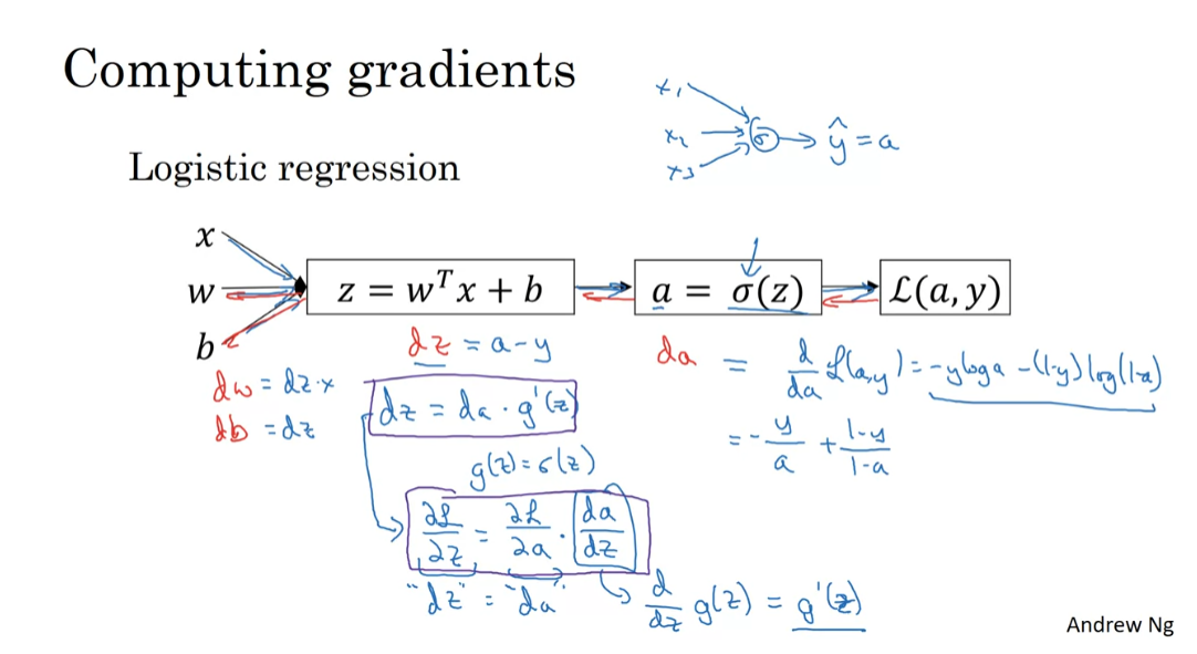
the whole works either way. Recall that when we talked
about logistic regression, we had this forward pass
where we compute z, then A, and then A loss and the
to take derivatives we had this backward
pass where we can first compute da and then
go on to compute dz, and then go on to
compute dw and db. The definition for the loss
was L of a comma y equals negative y log A minus 1
minus y times log 1 minus A. If you’re familiar with calculus and you take
the derivative of this with respect to A that will give you
the formula for da. So da is equal to that.

If you actually figure
out the calculus, you can show that this is negative y over A plus 1
minus y over one minus A. Just kind of derived that from calculus by taking
derivatives of this. It turns out when you take another step backwards
to compute dz, we then worked out
that dz is equal to A minus y. I didn’t
explain why previously, but it turns out that from
the chain rule of calculus, dz is equal to da
times g prime of z. Where here g of z
equals sigmoid of z as our activation function for this output unit in
logistic regression. Just remember, this is
still logistic regression, will have X_1, X_2, X_3, and then just
one sigmoid unit, and then that gives
us a, gives us y hat. Here the activation function
was sigmoid function. As an aside, only for
those of you familiar with the chain rule of calculus. The reason for this is because a is equal
to sigmoid of z, and so partial of L with respect to z is equal to partial of L with respect to
a times da, dz. Since A is equal
to sigmoid of z. This is equal to d, dz g of z, which is equal to g prime of z. That’s why this expression, which is dz in our code is
equal to this expression, which is da in our code
times g prime of z and so this just that. That last derivation would
have made sense only if you’re familiar with calculus and specifically the chain
rule from calculus. But if not, don’t
worry about it, I’ll try to explain the
intuition wherever it’s needed.

Then finally, having computed
dz for logistic regression, we will compute dw, which it turned out
was dz times x and db which is just dz where you have a
single training example. That was logistic regression.

What we’re going to
do when computing back-propagation for
a neural network is a calculation
a lot like this, but only we’ll do it twice. Because now we have not x
going to an output unit, but x going to a hidden layer and then going to
an output unit. Instead of this computation being one step as we have here, we’ll have two steps here in this neural network
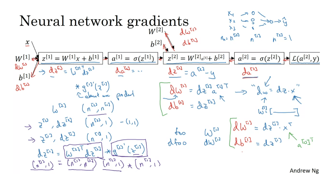
with two layers. In this two-layer
neural network, that is with the input layer, hidden layer, and
an output layer. Remember the steps
of a computation. First, you compute z_1 using this equation
and then compute a_1, and then you compute z_2. Notice z_2 also depends on
the parameters W_2 and b_2, and then based on
z_2 you compute a_2.

Then finally, that
gives you the loss. What back-propagation does,
is it will go backward to compute da_2 and then dz_2, then go back to
compute dW_2 and db_2. Go back to compute da_1, dz_1, and so on. We don’t need to take derivatives with
respect to the input x, since input x for supervised
learning because We’re not trying to optimize x, so we won’t bother
to take derivatives, at least for supervised
learning with respect to x. I’m going to skip
explicitly computing da. If you want, you can
actually compute da^2, and then use that
to compute dz^2. But in practice, you
could collapse both of these steps into one step. You end up that dz^2 is
equal to a^2 minus y, same as before, and
you have also going to write dw^2 and db^2
down here below. You have that dw^2 is equal
to dz^2 times a^1 transpose, and db^2 equals dz^2. This step is quite similar
for logistic regression, where we had that dw was
equal to dz times x, except that now, a^1
plays the role of x, and there’s an extra
transpose there. Because the relationship between the capital matrix W and our individual
parameters w was, there’s a transpose there, because w is equal
to a row vector. In the case of
logistic regression with the single output, dw^2 is like that, whereas
w here was a column vector. That’s why there’s an
extra transpose for a^1, whereas we didn’t for x here
for logistic regression. This completes half
of backpropagation. Then again, you
can compute da^1, if you wish although
in practice, the computation for da^1, and dz^1 are usually
collapsed into one step.

What you’d actually implement
is that dz^1 is equal to w^2 transpose times
dz^2 and then, times an element-wise
product of g^1 prime of z^1. Just to do a check
on the dimensions. If you have a neural network
that looks like this, outputs y if so. If you have n^0
and x equals n^0, and for features,
n^1 hidden units, and n^2 so far, and n^2 in our case, just one output unit, then the matrix w^2 is
n^2 by n^1 dimensional, z^2, and therefore,
dz^2 are going to be n^2 by one-dimensional. There’s really going
to be a one by one when we’re doing
binary classification, and z^1, and therefore also dz^1 are going to be n^1
by one-dimensional.

Note that for any variable, foo and dfoo always have
the same dimensions. That’s why, w and dw always
have the same dimension. Similarly, for b and db, and z and dz, and so on. To make sure that the dimensions
of these all match up, we have that dz^1 is equal to
w^2 transpose, times dz^2. Then, this is an
element-wise product times g^1 prime of z^1. Mashing the dimensions
from above, this is going to be n^1 by 1, is equal to w^2 transpose, we transpose of this. It is just going to be,
n^1 by n^2-dimensional, dz^2 is going to be n^2
by one-dimensional. Then, this is same
dimension as z^. This is also, n^1 by one-dimensional, so
element-wise product. The dimensions do make sense. N^1 by one-dimensional
vector can be obtained by n^1 by n^2
dimensional matrix, times n^2 by n^1, because the product of
these two things gives you an n^1 by
one-dimensional matrix. This becomes the
element-wise product of 2, n^1 by one-dimensional vectors, so the dimensions do match up. One tip when
implementing backprop, if you just make sure
that the dimensions of your matrices match up,
if you think through, what are the dimensions of your various matrices
including w^1, w^2, z^1, z^2, a^1, a^2, and so on, and just make sure that the dimensions of these matrix
operations may match up, sometimes that will already eliminate quite a lot
of bugs in backprop. This gives us dz^1.

Then finally, just to wrap up, dw^1 and db^1, we should write
them here, I guess. But since I’m running
out of space, I’ll write them on the
right of the slide, dw^1 and db^1 are given by
the following formulas. This is going to equal to
dz^1 times x transpose, and this is going
to be equal to dz. You might notice a
similarity between these equations and
these equations, which is really no coincidence, because x plays the role of a^0. X transpose is a^0 transpose. Those equations are
actually very similar. That gives a sense for how
backpropagation is derived.

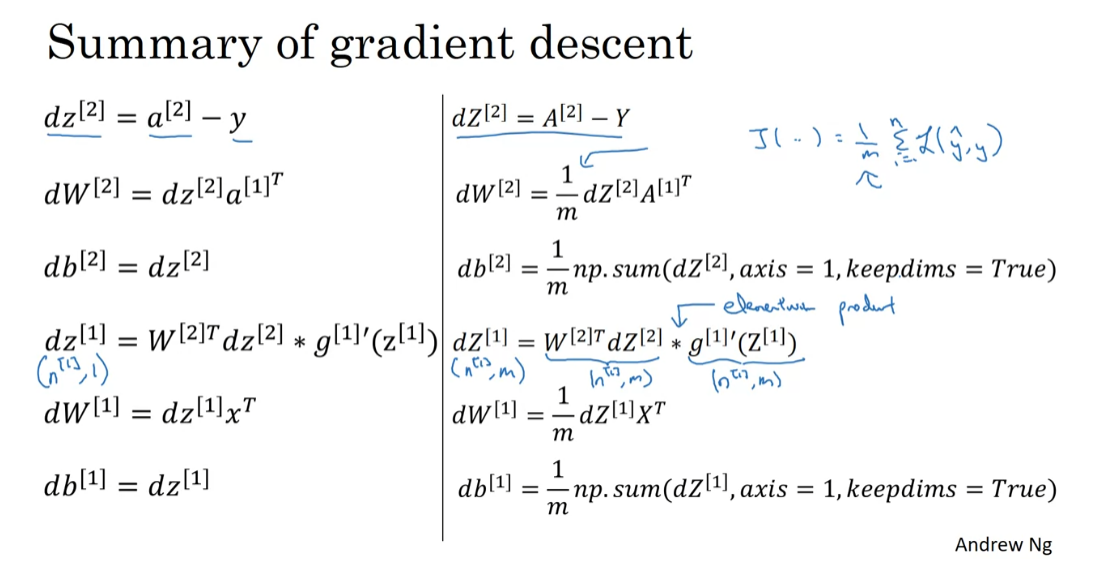
We have six key
equations here for dz_2, dw_2, db_2, dz_1,
dw_1, and db_1. Let me just take these
six equations and copy them over to
the next slide. Here they are. So
far we’ve derived that propagation for training on a single training
example at a time. But it should come
as no surprise that rather than working on a
single example at a time, we would like to vectorize across different
training examples.

vectorize

You remember that for a propagation when we’re operating on one
example at a time, we had equations like this, as well as say a^1
equals g^1 plus z^1. In order to vectorize,
we took say, the z’s and stack them
up in columns like this, z^1m, and call this capital Z. Then we found that by
stacking things up in columns and defining the capital
uppercase version of these, we then just had z^1
equals to the w^1x plus b and a^1 equals g^1 of z^1. We defined the notation
very carefully in this course to make sure that stacking examples into
different columns of a matrix makes
all this workout. It turns out that if you go
through the math carefully, the same trick also works
for backpropagation.

The vectorized equations
are as follows. First, if you take this dzs for different training
examples and stack them as different
columns of a matrix, same for this, same for this. Then this is the
vectorized implementation. Here’s how you can compute dW^2. There is this extra 1 over n because the cost function J is this 1 over m of the sum from I equals 1 through
m of the losses. When computing derivatives, we have that extra 1 over m term, just as we did when we were computing the weight updates
for logistic regression. That’s the update
you get for db^2, again, some of the dz’s. Then, we have 1 over m. Dz^1
is computed as follows. Once again, this is an
element-wise product only, whereas previously, we saw on the previous slide that this was an n1 by one-dimensional vector. No w, this is n1 by m
dimensional matrix. Both of these are also
n1 by m dimensional. That’s why that asterisk is
the element-wise product. Finally, the
remaining two updates perhaps shouldn’t
look too surprising.

I hope that gives you
some intuition for how the backpropagation
algorithm is derived. In all of machine learning, I think the derivation of the
backpropagation algorithm is actually one of the most complicated pieces
of math I’ve seen. It requires knowing both
linear algebra as well as the derivative of
matrices to really derive it from scratch
from first principles. If you are an expert
in matrix calculus, using this process, you might want to derive
the algorithm yourself. But I think that there
actually plenty of deep learning practitioners
that have seen the derivation at
about the level you’ve seen in this video
and are already able to have all the right
intuitions and be able to implement this algorithm
very effectively. If you are an expert in calculus do see if you can derive the
whole thing from scratch. It is one of the hardest
pieces of math on the very hardest derivations that I’ve seen in all
of machine learning. But either way, if
you implement this, this will work and
I think you have enough intuitions to tune
in and get it to work.

There’s just one last detail, my share of you before you
implement your neural network, which is how to initialize the weights
of your neural network. It turns out that initializing your
parameters not to zero, but randomly turns out to be very important for training
your neural network. In the next video,
you’ll see why.

Random Initialization

When you change your neural network, it’s important to initialize
the weights randomly. For logistic regression, it was okay
to initialize the weights to zero. But for a neural network of initialize
the weights to parameters to all zero and then applied gradient descent,
it won’t work. Let’s see why. So you have here two input features, so n0=2, and two hidden units, so n1=2. And so the matrix associated
with the hidden layer, w 1, is going to be two-by-two. Let’s say that you initialize it to
all 0s, so 0 0 0 0, two-by-two matrix. And let’s say B1 is also equal to 0 0. It turns out initializing the bias
terms b to 0 is actually okay, but initializing w to all 0s is a problem. So the problem with this
formalization is that for any example you give it,
you’ll have that a1,1 and a1,2, will be equal, right? So this activation and
this activation will be the same, because both of these hidden units
are computing exactly the same function. And then,
when you compute backpropagation, it turns out that dz11 and dz12 will also be the same
colored by symmetry, right? Both of these hidden units
will initialize the same way. Technically, for what I’m saying, I’m assuming that the outgoing weights or
also identical. So that’s w2 is equal to 0 0. But if you initialize
the neural network this way, then this hidden unit and
this hidden unit are completely identical.

Sometimes you say they’re
completely symmetric, which just means that they’re
completing exactly the same function. And by kind of a proof by induction, it turns out that after every single
iteration of training your two hidden units are still computing
exactly the same function. Since plots will show that dw will
be a matrix that looks like this. Where every row takes on the same value. So we perform a weight update. So when you perform a weight update,
w1 gets updated as w1- alpha times dw. You find that w1, after every iteration, will have the first row
equal to the second row. So it’s possible to construct
a proof by induction that if you initialize all the ways,
all the values of w to 0, then because both hidden units start
off computing the same function. And both hidden the units have
the same influence on the output unit, then after one iteration,
that same statement is still true, the two hidden units are still symmetric. And therefore, by induction, after two
iterations, three iterations and so on, no matter how long you
train your neural network, both hidden units are still
computing exactly the same function. And so in this case, there’s really no
point to having more than one hidden unit. Because they are all
computing the same thing.

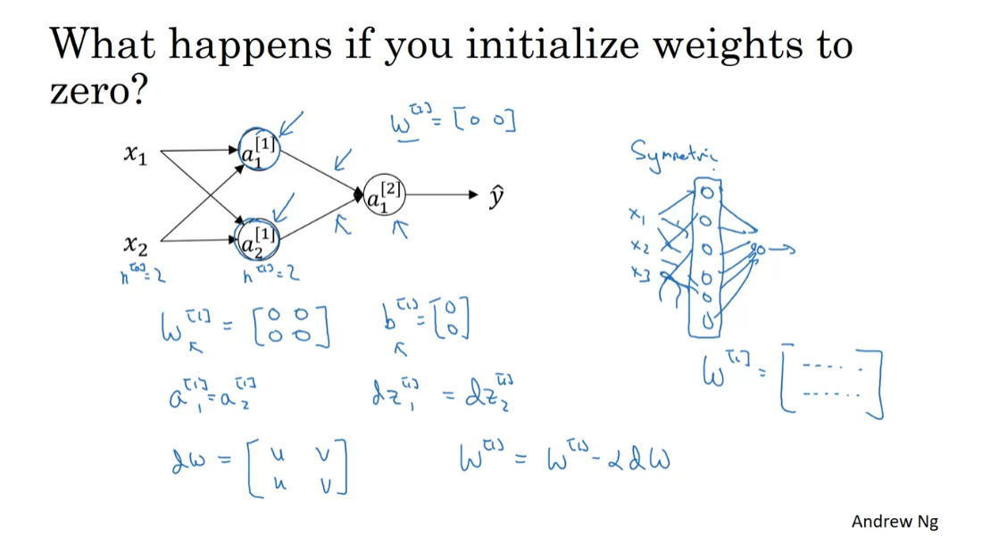
And of course, for larger neural networks,
let’s say of three features and maybe a very large number of hidden units, a similar argument works to show that
with a neural network like this. Let me draw all the edges,
if you initialize the weights to zero, then all of your hidden
units are symmetric. And no matter how long
you’re upgrading the center, all continue to compute
exactly the same function. So that’s not helpful,
because you want the different hidden units to compute
different functions.

The solution to this is to
initialize your parameters randomly. So here’s what you do. You can set w1 = np.random.randn. This generates a gaussian
random variable (2,2). And then usually, you multiply this
by very small number, such as 0.01. So you initialize it to
very small random values. And then b, it turns out that b
does not have the symmetry problem, what’s called the symmetry
breaking problem. So it’s okay to initialize
b to just zeros. Because so
long as w is initialized randomly, you start off with the different hidden
units computing different things. And so you no longer have this
symmetry breaking problem. And then similarly, for w2,
you’re going to initialize that randomly. And b2, you can initialize that to 0. So you might be wondering, where did this
constant come from and why is it 0.01? Why not put the number 100 or 1000? Turns out that we usually
prefer to initialize the weights to very small random values. Because if you are using a tanh or
sigmoid activation function, or the other sigmoid,
even just at the output layer. If the weights are too large, then when you compute
the activation values, remember that z[1]=w1 x + b. And then a1 is the activation
function applied to z1. So if w is very big,
z will be very, or at least some values of z will be either very large or
very small. And so in that case, you’re more likely
to end up at these fat parts of the tanh function or the sigmoid function, where
the slope or the gradient is very small. Meaning that gradient
descent will be very slow. So learning was very slow.

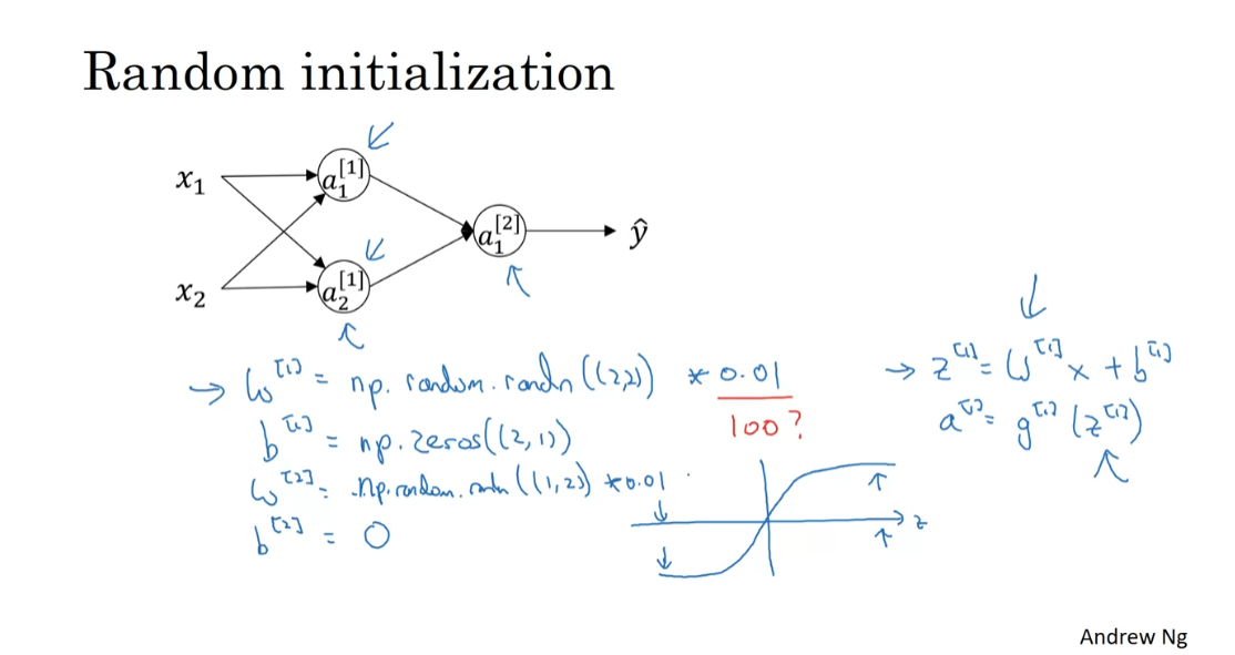
So just a recap, if w is too large,
you’re more likely to end up even at the very start of training,
with very large values of z. Which causes your tanh or your sigmoid
activation function to be saturated, thus slowing down learning. If you don’t have any sigmoid or tanh activation functions throughout your
neural network, this is less of an issue. But if you’re doing binary classification,
and your output unit is a sigmoid function, then you just don’t want
the initial parameters to be too large. So that’s why multiplying by 0.01 would
be something reasonable to try, or any other small number. And same for w2, right? This can be random.random. I guess this would be 1 by 2
in this example, times 0.01. Missing an s there. So finally, it turns out that sometimes
they can be better constants than 0.01. When you’re training a neural
network with just one hidden layer, it is a relatively shallow neural network,
without too many hidden layers. Set it to 0.01 will probably work okay. But when you’re training a very
very deep neural network, then you might want to pick
a different constant than 0.01.

And in next week’s material,
we’ll talk a little bit about how and when you might want to choose
a different constant than 0.01. But either way, it will usually end
up being a relatively small number. So that’s it for this week’s videos. You now know how to set up a neural
network of a hidden layer, initialize the parameters,
make predictions using. As well as compute derivatives and
implement gradient descent, using backprop. So that,
you should be able to do the quizzes, as well as this week’s
programming exercises. Best of luck with that. I hope you have fun with
the problem exercise, and look forward to seeing you
in the week four materials.

神经网络的权重需要随机初始化，而不是初始化为零，主要有以下几个原因：

1. 破坏对称性： 如果所有权重都初始化为相同的值，那么每个神经元在前向传播过程中会得到相同的输入，导致它们学习相同的特征。这会使网络失去表达能力，因为每一层的神经元都会进行相同的计算，无法提取有效的特征。

2. 避免梯度对称性： 如果所有权重都初始化为零，那么每个神经元的梯度也会相同。这样在反向传播过程中，所有权重都会更新为相同的值，这种对称性会导致网络无法收敛到有效的解决方案。

3. 增加网络的多样性： 通过随机初始化权重，可以增加网络的多样性，使得不同的神经元可以学习不同的特征。这样可以增强网络的表达能力，使其能够更好地适应复杂的数据分布。

4. 避免陷入局部最优解： 随机初始化权重可以帮助神经网络避免陷入局部最优解。如果所有权重都初始化为相同的值，那么所有神经元都会沿着相同的梯度方向移动，导致网络可能陷入局部最优解而无法找到全局最优解。

因此，通过随机初始化权重，可以打破对称性，增加网络的多样性，避免梯度对称性，并且帮助网络避免陷入局部最优解，从而提高神经网络的学习效果和泛化能力。

Quiz: Shallow Neural Networks

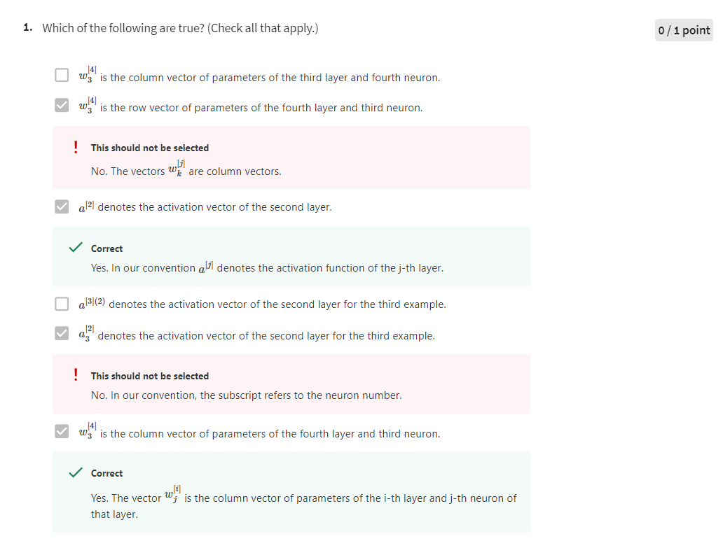
做第二遍还是错

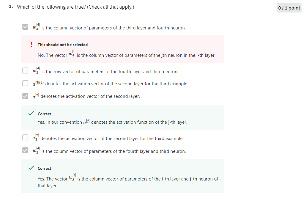
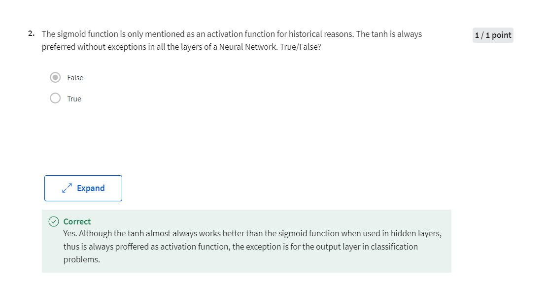
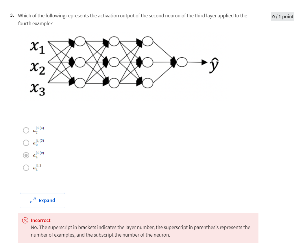
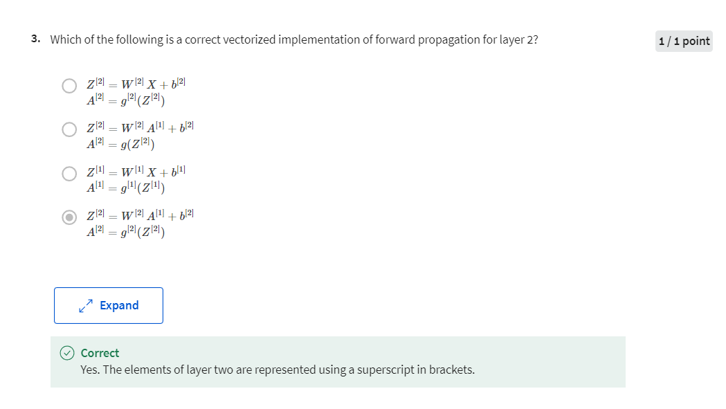
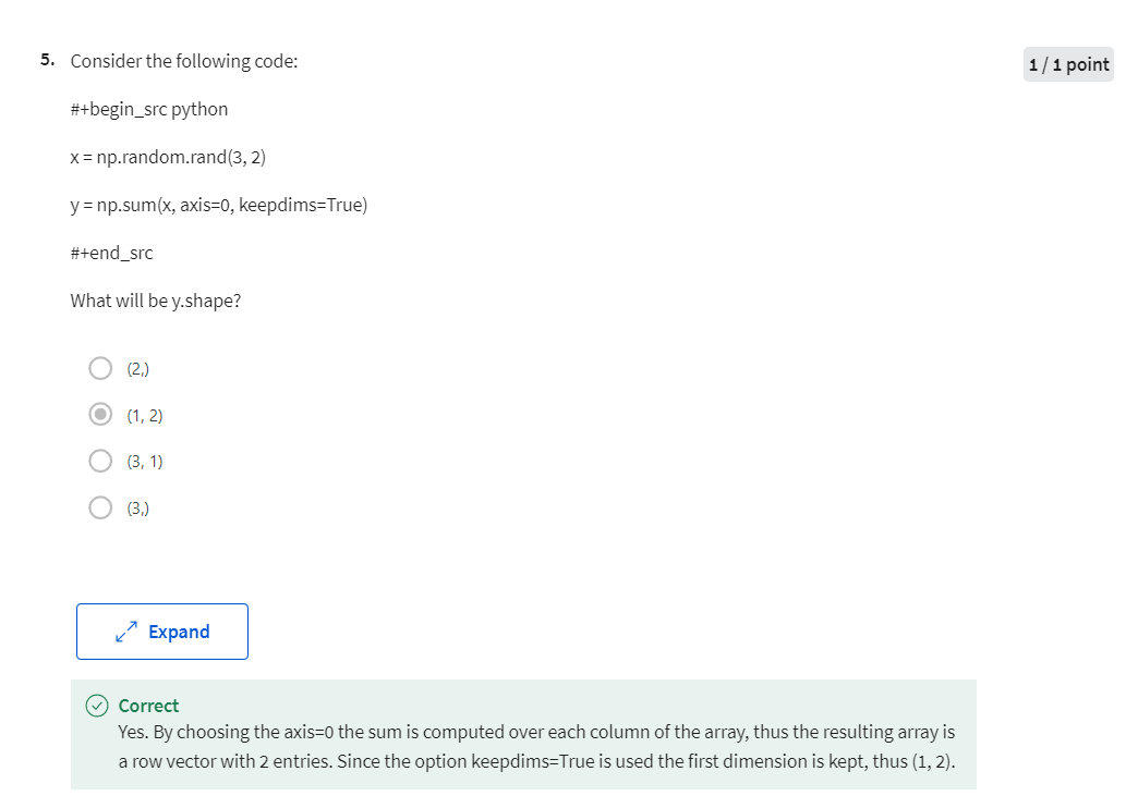
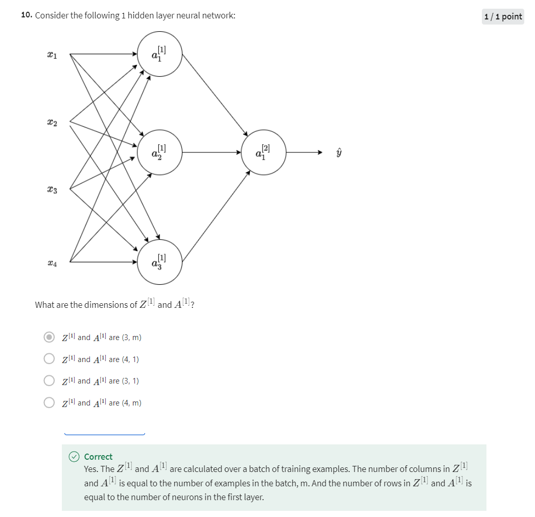
Programming Assignment: Planar Data Classification with One Hidden Layer

Planar data classification with one hidden layer

Welcome to your week 3 programming assignment! It’s time to build your first neural network, which will have one hidden layer. Now, you’ll notice a big difference between this model and the one you implemented previously using logistic regression.

By the end of this assignment, you’ll be able to:

• Implement a 2-class classification neural network with a single hidden layer
• Use units with a non-linear activation function, such as tanh
• Compute the cross entropy loss
• Implement forward and backward propagation

Important Note on Submission to the AutoGrader

Before submitting your assignment to the AutoGrader, please make sure you are not doing the following:

1. You have not added any extra print statement(s) in the assignment.
2. You have not added any extra code cell(s) in the assignment.
3. You have not changed any of the function parameters.
4. You are not using any global variables inside your graded exercises. Unless specifically instructed to do so, please refrain from it and use the local variables instead.
5. You are not changing the assignment code where it is not required, like creating extra variables.

If you do any of the following, you will get something like, Grader Error: Grader feedback not found (or similarly unexpected) error upon submitting your assignment. Before asking for help/debugging the errors in your assignment, check for these first. If this is the case, and you don’t remember the changes you have made, you can get a fresh copy of the assignment by following these instructions.

1 - Packages

First import all the packages that you will need during this assignment.

• numpy is the fundamental package for scientific computing with Python.
• sklearn provides simple and efficient tools for data mining and data analysis.
• matplotlib is a library for plotting graphs in Python.
• testCases provides some test examples to assess the correctness of your functions
• planar_utils provide various useful functions used in this assignment

# Package imports
import numpy as np
import copy
import matplotlib.pyplot as plt
from testCases_v2 import *
from public_tests import *
import sklearn
import sklearn.datasets
import sklearn.linear_model
from planar_utils import plot_decision_boundary, sigmoid, load_planar_dataset, load_extra_datasets

%matplotlib inline

%load_ext autoreload
%autoreload 2

2 - Load the Dataset

X, Y = load_planar_dataset()

Visualize the dataset using matplotlib. The data looks like a “flower” with some red (label y=0) and some blue (y=1) points. Your goal is to build a model to fit this data. In other words, we want the classifier to define regions as either red or blue.

# Visualize the data:
plt.scatter(X[0, :], X[1, :], c=Y, s=40, cmap=plt.cm.Spectral);

Output

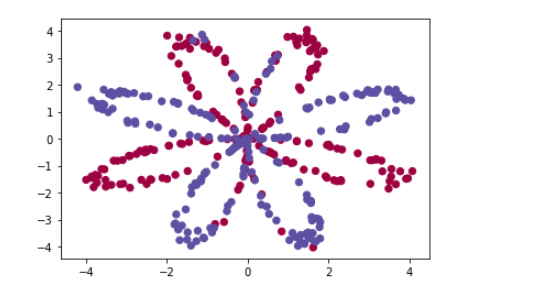
You have:
- a numpy-array (matrix) X that contains your features (x1, x2)
- a numpy-array (vector) Y that contains your labels (red:0, blue:1).

First, get a better sense of what your data is like.

Exercise 1

How many training examples do you have? In addition, what is the shape of the variables X and Y?

Hint: How do you get the shape of a numpy array? (help)

# (≈ 3 lines of code)
# shape_X = ...
# shape_Y = ...
# training set size
# m = ...
# YOUR CODE STARTS HERE
shape_X = X.shape
shape_Y = Y.shape
m = X.shape[1]

# YOUR CODE ENDS HERE

print ('The shape of X is: ' + str(shape_X))
print ('The shape of Y is: ' + str(shape_Y))
print ('I have m = %d training examples!' % (m))

Output

The shape of X is: (2, 400)
The shape of Y is: (1, 400)
I have m = 400 training examples!

3 - Simple Logistic Regression

Before building a full neural network, let’s check how logistic regression performs on this problem. You can use sklearn’s built-in functions for this. Run the code below to train a logistic regression classifier on the dataset.

# Train the logistic regression classifier
clf = sklearn.linear_model.LogisticRegressionCV();
clf.fit(X.T, Y.T);

You can now plot the decision boundary of these models! Run the code below.

# Plot the decision boundary for logistic regression
plot_decision_boundary(lambda x: clf.predict(x), X, Y)
plt.title("Logistic Regression")

# Print accuracy
LR_predictions = clf.predict(X.T)
print ('Accuracy of logistic regression: %d ' % float((np.dot(Y,LR_predictions) + np.dot(1-Y,1-LR_predictions))/float(Y.size)*100) +
       '% ' + "(percentage of correctly labelled datapoints)")

Output

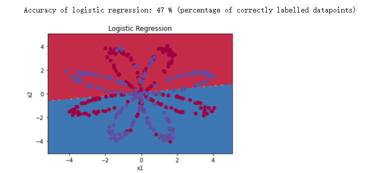
Interpretation: The dataset is not linearly separable, so logistic regression doesn’t perform well. Hopefully a neural network will do better. Let’s try this now!

4 - Neural Network model

Logistic regression didn’t work well on the flower dataset. Next, you’re going to train a Neural Network with a single hidden layer and see how that handles the same problem.

The model:

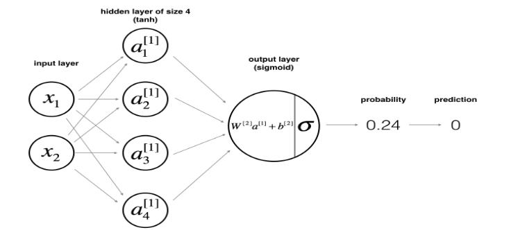
Mathematically:

For one example $x^{(i)}$:
$$z^{[1](i)}=W^{[1]}{x}^{(i)}+b^{[1]}\text{\hspace{1em}(1)}$$
$$a^{[1](i)}=\tanh (z^{[1](i)})\text{\hspace{1em}(2)}$$
$$z^{[2](i)}=W^{[2]}{a}^{[1](i)}+b^{[2]}\text{\hspace{1em}(3)}$$
$${\hat{y}}^{(i)}=a^{[2](i)}=\sigma (z^{[2](i)})\text{\hspace{1em}(4)}$$
$$y_{prediction}^{(i)}=\{\begin{array}{ll}1& if{a}^{[2](i)}>0.5\\ 0& otherwise\end{array}\text{\hspace{1em}(5)}$$

Given the predictions on all the examples, you can also compute the cost $J$ as follows:

$$J=-\frac{1}{m}\sum _{i=1}^m\left(y^{(i)}\log (a^{[2](i)})+(1-y^{(i)})\log (1-a^{[2](i)})\right)$$

Reminder: The general methodology to build a Neural Network is to:
1. Define the neural network structure ( # of input units, # of hidden units, etc).
2. Initialize the model’s parameters
3. Loop:
- Implement forward propagation
- Compute loss
- Implement backward propagation to get the gradients
- Update parameters (gradient descent)

In practice, you’ll often build helper functions to compute steps 1-3, then merge them into one function called nn_model(). Once you’ve built nn_model() and learned the right parameters, you can make predictions on new data.

4.1 - Defining the neural network structure

Exercise 2 - layer_sizes

Define three variables:

• n_x: the size of the input layer
• n_h: the size of the hidden layer (set this to 4, as n_h = 4, but only for this Exercise 2)
• n_y: the size of the output layer

Hint: Use shapes of X and Y to find n_x and n_y. Also, hard code the hidden layer size to be 4.

# GRADED FUNCTION: layer_sizes

def layer_sizes(X, Y):
    """
    Arguments:
    X -- input dataset of shape (input size, number of examples)
    Y -- labels of shape (output size, number of examples)
    
    Returns:
    n_x -- the size of the input layer
    n_h -- the size of the hidden layer
    n_y -- the size of the output layer
    """
    #(≈ 3 lines of code)
    # n_x = ... 
    # n_h = ...
    # n_y = ... 
    # YOUR CODE STARTS HERE
    n_x = X.shape[0]
    n_h = 4
    n_y = Y.shape[0]
    
    # YOUR CODE ENDS HERE
    return (n_x, n_h, n_y)

t_X, t_Y = layer_sizes_test_case()
(n_x, n_h, n_y) = layer_sizes(t_X, t_Y)
print("The size of the input layer is: n_x = " + str(n_x))
print("The size of the hidden layer is: n_h = " + str(n_h))
print("The size of the output layer is: n_y = " + str(n_y))

layer_sizes_test(layer_sizes)

Output

The size of the input layer is: n_x = 5
The size of the hidden layer is: n_h = 4
The size of the output layer is: n_y = 2
All tests passed!

Expected output

The size of the input layer is: n_x = 5
The size of the hidden layer is: n_h = 4
The size of the output layer is: n_y = 2
All tests passed!

4.2 - Initialize the model’s parameters

Exercise 3 - initialize_parameters

Implement the function initialize_parameters().

Instructions:

• Make sure your parameters’ sizes are right. Refer to the neural network figure above if needed.
• You will initialize the weights matrices with random values.
  • Use: np.random.randn(a,b) * 0.01 to randomly initialize a matrix of shape (a,b).
• You will initialize the bias vectors as zeros.
  • Use: np.zeros((a,b)) to initialize a matrix of shape (a,b) with zeros.

# GRADED FUNCTION: initialize_parameters

def initialize_parameters(n_x, n_h, n_y):
    """
    Argument:
    n_x -- size of the input layer
    n_h -- size of the hidden layer
    n_y -- size of the output layer
    
    Returns:
    params -- python dictionary containing your parameters:
                    W1 -- weight matrix of shape (n_h, n_x)
                    b1 -- bias vector of shape (n_h, 1)
                    W2 -- weight matrix of shape (n_y, n_h)
                    b2 -- bias vector of shape (n_y, 1)
    """    
    #(≈ 4 lines of code)
    # W1 = ...
    # b1 = ...
    # W2 = ...
    # b2 = ...
    # YOUR CODE STARTS HERE
    W1 = np.random.randn(n_h, n_x) * 0.01
    b1 = np.zeros((n_h, 1))
    W2 = np.random.randn(n_y, n_h) * 0.01
    b2 = np.zeros((n_y, 1))
    
    # YOUR CODE ENDS HERE

    parameters = {"W1": W1,
                  "b1": b1,
                  "W2": W2,
                  "b2": b2}
    
    return parameters

np.random.seed(2)
n_x, n_h, n_y = initialize_parameters_test_case()
parameters = initialize_parameters(n_x, n_h, n_y)

print("W1 = " + str(parameters["W1"]))
print("b1 = " + str(parameters["b1"]))
print("W2 = " + str(parameters["W2"]))
print("b2 = " + str(parameters["b2"]))

initialize_parameters_test(initialize_parameters)

Output

W1 = [[-0.00416758 -0.00056267]
 [-0.02136196  0.01640271]
 [-0.01793436 -0.00841747]
 [ 0.00502881 -0.01245288]]
b1 = [[0.]
 [0.]
 [0.]
 [0.]]
W2 = [[-0.01057952 -0.00909008  0.00551454  0.02292208]]
b2 = [[0.]]
All tests passed!

Expected output

W1 = [[-0.00416758 -0.00056267]
 [-0.02136196  0.01640271]
 [-0.01793436 -0.00841747]
 [ 0.00502881 -0.01245288]]
b1 = [[0.]
 [0.]
 [0.]
 [0.]]
W2 = [[-0.01057952 -0.00909008  0.00551454  0.02292208]]
b2 = [[0.]]
All tests passed!

4.3 - The Loop

Exercise 4 - forward_propagation

Implement forward_propagation() using the following equations:

$$Z^{[1]}=W^{[1]}X+b^{[1]}\text{\hspace{1em}(1)}$$
$$A^{[1]}=\tanh (Z^{[1]})\text{\hspace{1em}(2)}$$
$$Z^{[2]}=W^{[2]}{A}^{[1]}+b^{[2]}\text{\hspace{1em}(3)}$$
$$\hat{Y}=A^{[2]}=\sigma (Z^{[2]})\text{\hspace{1em}(4)}$$

Instructions:

• Check the mathematical representation of your classifier in the figure above.
• Use the function sigmoid(). It’s built into (imported) this notebook.
• Use the function np.tanh(). It’s part of the numpy library.
• Implement using these steps:
  1. Retrieve each parameter from the dictionary “parameters” (which is the output of initialize_parameters() by using parameters[".."].
  2. Implement Forward Propagation. Compute $Z^{[1]},A^{[1]},Z^{[2]}$ and $A^{[2]}$ (the vector of all your predictions on all the examples in the training set).
• Values needed in the backpropagation are stored in “cache”. The cache will be given as an input to the backpropagation function.

# GRADED FUNCTION:forward_propagation

def forward_propagation(X, parameters):
    """
    Argument:
    X -- input data of size (n_x, m)
    parameters -- python dictionary containing your parameters (output of initialization function)
    
    Returns:
    A2 -- The sigmoid output of the second activation
    cache -- a dictionary containing "Z1", "A1", "Z2" and "A2"
    """
    # Retrieve each parameter from the dictionary "parameters"
    #(≈ 4 lines of code)
    # W1 = ...
    # b1 = ...
    # W2 = ...
    # b2 = ...
    # YOUR CODE STARTS HERE
    W1 = parameters["W1"]
    b1 = parameters["b1"]
    W2 = parameters["W2"]
    b2 = parameters["b2"]
    
    # YOUR CODE ENDS HERE
    
    # Implement Forward Propagation to calculate A2 (probabilities)
    # (≈ 4 lines of code)
    # Z1 = ...
    # A1 = ...
    # Z2 = ...
    # A2 = ...
    # YOUR CODE STARTS HERE
    Z1 = np.dot(W1, X) + b1
    A1 = np.tanh(Z1)
    Z2 = np.dot(W2, A1) + b2
    A2 = sigmoid(Z2)
    
    # YOUR CODE ENDS HERE
    
    assert(A2.shape == (1, X.shape[1]))
    
    cache = {"Z1": Z1,
             "A1": A1,
             "Z2": Z2,
             "A2": A2}
    
    return A2, cache

t_X, parameters = forward_propagation_test_case()
A2, cache = forward_propagation(t_X, parameters)
print("A2 = " + str(A2))

forward_propagation_test(forward_propagation)

Output

A2 = [[0.21292656 0.21274673 0.21295976]]
All tests passed!

Expected output

A2 = [[0.21292656 0.21274673 0.21295976]]
All tests passed!

4.4 - Compute the Cost

Now that you’ve computed $A^{[2]}$ (in the Python variable “A2”), which contains $a^{[2](i)}$ for all examples, you can compute the cost function as follows:

$$J=-\frac{1}{m}\sum _{i=1}^m(y^{(i)}\log \left(a^{[2](i)}\right)+(1-y^{(i)})\log \left(1-a^{[2](i)}\right))\text{\hspace{1em}(13)}$$

Exercise 5 - compute_cost

Implement compute_cost() to compute the value of the cost $J$.

Instructions:

• There are many ways to implement the cross-entropy loss. This is one way to implement one part of the equation without for loops:
  $-\sum _{i=1}^m{y}^{(i)}\log (a^{[2](i)})$:

logprobs = np.multiply(np.log(A2),Y)
cost = - np.sum(logprobs)          

• Use that to build the whole expression of the cost function.

Notes:

• You can use either np.multiply() and then np.sum() or directly np.dot()).
• If you use np.multiply followed by np.sum the end result will be a type float, whereas if you use np.dot, the result will be a 2D numpy array.
• You can use np.squeeze() to remove redundant dimensions (in the case of single float, this will be reduced to a zero-dimension array).
• You can also cast the array as a type float using float().

# GRADED FUNCTION: compute_cost

def compute_cost(A2, Y):
    """
    Computes the cross-entropy cost given in equation (13)
    
    Arguments:
    A2 -- The sigmoid output of the second activation, of shape (1, number of examples)
    Y -- "true" labels vector of shape (1, number of examples)

    Returns:
    cost -- cross-entropy cost given equation (13)
    
    """
    
    m = Y.shape[1] # number of examples

    # Compute the cross-entropy cost
    # (≈ 2 lines of code)
    # logprobs = ...
    # cost = ...
    # YOUR CODE STARTS HERE
    logprobs = np.multiply(np.log(A2), Y) + np.multiply(1 - Y, np.log(1 - A2))
    cost = - 1 / m * np.sum(logprobs)
    
    # YOUR CODE ENDS HERE
    
    cost = float(np.squeeze(cost))  # makes sure cost is the dimension we expect. 
                                    # E.g., turns [[17]] into 17 
    
    return cost

A2, t_Y = compute_cost_test_case()
cost = compute_cost(A2, t_Y)
print("cost = " + str(compute_cost(A2, t_Y)))

compute_cost_test(compute_cost)

Output

cost = 0.6930587610394646
All tests passed!

Expected output

cost = 0.6930587610394646
All tests passed!

4.5 - Implement Backpropagation

Using the cache computed during forward propagation, you can now implement backward propagation.

Exercise 6 - backward_propagation

Implement the function backward_propagation().

Instructions:
Backpropagation is usually the hardest (most mathematical) part in deep learning. To help you, here again is the slide from the lecture on backpropagation. You’ll want to use the six equations on the right of this slide, since you are building a vectorized implementation.

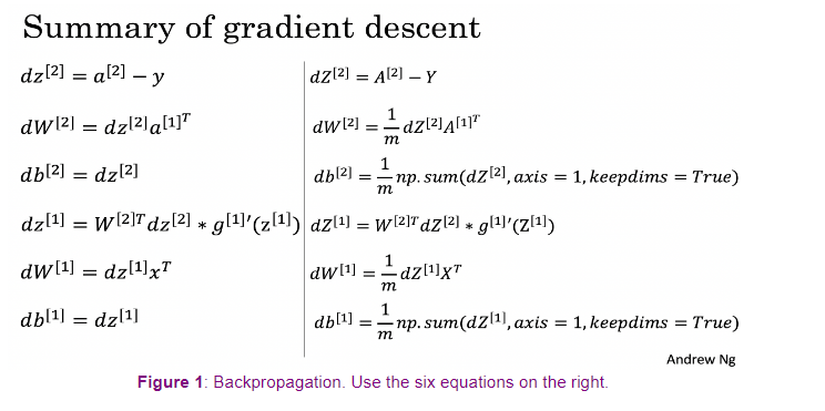
• Tips:
  • To compute dZ1 you’ll need to compute $g^{[1{]}^{\prime }}(Z^{[1]})$. Since $g^{[1]}(.)$ is the tanh activation function, if $a=g^{[1]}(z)$ then $g^{[1{]}^{\prime }}(z)=1-a^2$. So you can compute
    $g^{[1{]}^{\prime }}(Z^{[1]})$ using (1 - np.power(A1, 2)).

# GRADED FUNCTION: backward_propagation

def backward_propagation(parameters, cache, X, Y):
    """
    Implement the backward propagation using the instructions above.
    
    Arguments:
    parameters -- python dictionary containing our parameters 
    cache -- a dictionary containing "Z1", "A1", "Z2" and "A2".
    X -- input data of shape (2, number of examples)
    Y -- "true" labels vector of shape (1, number of examples)
    
    Returns:
    grads -- python dictionary containing your gradients with respect to different parameters
    """
    m = X.shape[1]
    
    # First, retrieve W1 and W2 from the dictionary "parameters".
    #(≈ 2 lines of code)
    # W1 = ...
    # W2 = ...
    # YOUR CODE STARTS HERE
    W1 = parameters["W1"]
    W2 = parameters["W2"]
    
    # YOUR CODE ENDS HERE
        
    # Retrieve also A1 and A2 from dictionary "cache".
    #(≈ 2 lines of code)
    # A1 = ...
    # A2 = ...
    # YOUR CODE STARTS HERE
    A1 = cache["A1"]
    A2 = cache["A2"]
    
    # YOUR CODE ENDS HERE
    
    # Backward propagation: calculate dW1, db1, dW2, db2. 
    #(≈ 6 lines of code, corresponding to 6 equations on slide above)
    # dZ2 = ...
    # dW2 = ...
    # db2 = ...
    # dZ1 = ...
    # dW1 = ...
    # db1 = ...
    # YOUR CODE STARTS HERE
    dZ2 = A2 - Y
    dW2 = 1 / m * np.dot(dZ2, A1.T)
    db2 = 1 / m * np.sum(dZ2, axis=1, keepdims=True)
    dZ1 = np.dot(W2.T, dZ2) * (1 - np.power(A1, 2))
    dW1 = 1 / m * np.dot(dZ1, X.T)
    db1 = 1 / m * np.sum(dZ1, axis=1, keepdims=True)
    
    
    # YOUR CODE ENDS HERE
    
    grads = {"dW1": dW1,
             "db1": db1,
             "dW2": dW2,
             "db2": db2}
    
    return grads

parameters, cache, t_X, t_Y = backward_propagation_test_case()

grads = backward_propagation(parameters, cache, t_X, t_Y)
print ("dW1 = "+ str(grads["dW1"]))
print ("db1 = "+ str(grads["db1"]))
print ("dW2 = "+ str(grads["dW2"]))
print ("db2 = "+ str(grads["db2"]))

backward_propagation_test(backward_propagation)

Output

dW1 = [[ 0.00301023 -0.00747267]
 [ 0.00257968 -0.00641288]
 [-0.00156892  0.003893  ]
 [-0.00652037  0.01618243]]
db1 = [[ 0.00176201]
 [ 0.00150995]
 [-0.00091736]
 [-0.00381422]]
dW2 = [[ 0.00078841  0.01765429 -0.00084166 -0.01022527]]
db2 = [[-0.16655712]]
All tests passed!

Expected output

dW1 = [[ 0.00301023 -0.00747267]
 [ 0.00257968 -0.00641288]
 [-0.00156892  0.003893  ]
 [-0.00652037  0.01618243]]
db1 = [[ 0.00176201]
 [ 0.00150995]
 [-0.00091736]
 [-0.00381422]]
dW2 = [[ 0.00078841  0.01765429 -0.00084166 -0.01022527]]
db2 = [[-0.16655712]]
All tests passed!

4.6 - Update Parameters

Exercise 7 - update_parameters

Implement the update rule. Use gradient descent. You have to use (dW1, db1, dW2, db2) in order to update (W1, b1, W2, b2).

General gradient descent rule: $\theta =\theta -\alpha \frac{\partial J}{\partial \theta }$ where $\alpha$ is the learning rate and $\theta$ represents a parameter.

Figure 2: The gradient descent algorithm with a good learning rate (converging) and a bad learning rate (diverging). Images courtesy of Adam Harley.

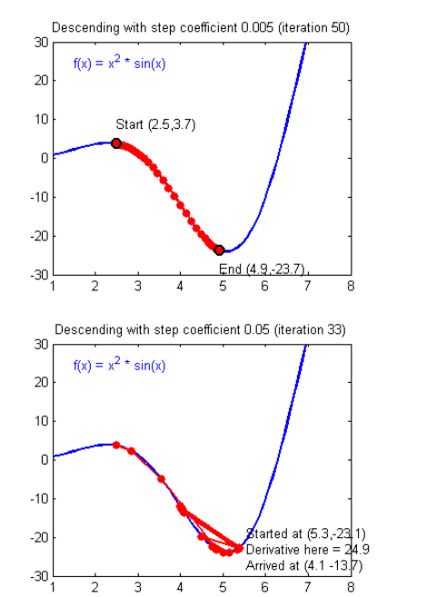
Hint

• Use copy.deepcopy(...) when copying lists or dictionaries that are passed as parameters to functions. It avoids input parameters being modified within the function. In some scenarios, this could be inefficient, but it is required for grading purposes.

# GRADED FUNCTION: update_parameters

def update_parameters(parameters, grads, learning_rate = 1.2):
    """
    Updates parameters using the gradient descent update rule given above
    
    Arguments:
    parameters -- python dictionary containing your parameters 
    grads -- python dictionary containing your gradients 
    
    Returns:
    parameters -- python dictionary containing your updated parameters 
    """
    # Retrieve a copy of each parameter from the dictionary "parameters". Use copy.deepcopy(...) for W1 and W2
    #(≈ 4 lines of code)
    # W1 = ...
    # b1 = ...
    # W2 = ...
    # b2 = ...
    # YOUR CODE STARTS HERE
    W1 = copy.deepcopy(parameters["W1"])
    b1 = parameters["b1"]
    W2 = copy.deepcopy(parameters["W2"])
    b2 = parameters["b2"]
    
    # YOUR CODE ENDS HERE
    
    # Retrieve each gradient from the dictionary "grads"
    #(≈ 4 lines of code)
    # dW1 = ...
    # db1 = ...
    # dW2 = ...
    # db2 = ...
    # YOUR CODE STARTS HERE
    dW1 = grads["dW1"]
    db1 = grads["db1"]
    dW2 = grads["dW2"]
    db2 = grads["db2"]
    
    # YOUR CODE ENDS HERE
    
    # Update rule for each parameter
    #(≈ 4 lines of code)
    # W1 = ...
    # b1 = ...
    # W2 = ...
    # b2 = ...
    # YOUR CODE STARTS HERE
    W1 = W1 - learning_rate * dW1
    b1 = b1 - learning_rate * db1
    W2 = W2 - learning_rate * dW2
    b2 = b2 - learning_rate * db2
    
    
    # YOUR CODE ENDS HERE
    
    parameters = {"W1": W1,
                  "b1": b1,
                  "W2": W2,
                  "b2": b2}
    
    return parameters

parameters, grads = update_parameters_test_case()
parameters = update_parameters(parameters, grads)

print("W1 = " + str(parameters["W1"]))
print("b1 = " + str(parameters["b1"]))
print("W2 = " + str(parameters["W2"]))
print("b2 = " + str(parameters["b2"]))

update_parameters_test(update_parameters)

Output

W1 = [[-0.00643025  0.01936718]
 [-0.02410458  0.03978052]
 [-0.01653973 -0.02096177]
 [ 0.01046864 -0.05990141]]
b1 = [[-1.02420756e-06]
 [ 1.27373948e-05]
 [ 8.32996807e-07]
 [-3.20136836e-06]]
W2 = [[-0.01041081 -0.04463285  0.01758031  0.04747113]]
b2 = [[0.00010457]]
All tests passed!

Expected output

W1 = [[-0.00643025  0.01936718]
 [-0.02410458  0.03978052]
 [-0.01653973 -0.02096177]
 [ 0.01046864 -0.05990141]]
b1 = [[-1.02420756e-06]
 [ 1.27373948e-05]
 [ 8.32996807e-07]
 [-3.20136836e-06]]
W2 = [[-0.01041081 -0.04463285  0.01758031  0.04747113]]
b2 = [[0.00010457]]
All tests passed!

4.7 - Integration

Integrate your functions in nn_model()

Exercise 8 - nn_model

Build your neural network model in nn_model().

Instructions: The neural network model has to use the previous functions in the right order.

# GRADED FUNCTION: nn_model

def nn_model(X, Y, n_h, num_iterations = 10000, print_cost=False):
    """
    Arguments:
    X -- dataset of shape (2, number of examples)
    Y -- labels of shape (1, number of examples)
    n_h -- size of the hidden layer
    num_iterations -- Number of iterations in gradient descent loop
    print_cost -- if True, print the cost every 1000 iterations
    
    Returns:
    parameters -- parameters learnt by the model. They can then be used to predict.
    """
    
    np.random.seed(3)
    n_x = layer_sizes(X, Y)[0]
    n_y = layer_sizes(X, Y)[2]
    
    # Initialize parameters
    #(≈ 1 line of code)
    # parameters = ...
    # YOUR CODE STARTS HERE
    parameters = initialize_parameters(n_x, n_h, n_y)
    
    # YOUR CODE ENDS HERE
    
    # Loop (gradient descent)

    for i in range(0, num_iterations):
         
        #(≈ 4 lines of code)
        # Forward propagation. Inputs: "X, parameters". Outputs: "A2, cache".
        # A2, cache = ...
        
        # Cost function. Inputs: "A2, Y". Outputs: "cost".
        # cost = ...
 
        # Backpropagation. Inputs: "parameters, cache, X, Y". Outputs: "grads".
        # grads = ...
 
        # Gradient descent parameter update. Inputs: "parameters, grads". Outputs: "parameters".
        # parameters = ...
        
        # YOUR CODE STARTS HERE
        A2, cache = forward_propagation(X, parameters)
        cost = compute_cost(A2, Y)
        grads = backward_propagation(parameters, cache, X, Y)
        parameters = update_parameters(parameters, grads)
        
        # YOUR CODE ENDS HERE
        
        # Print the cost every 1000 iterations
        if print_cost and i % 1000 == 0:
            print ("Cost after iteration %i: %f" %(i, cost))

    return parameters

nn_model_test(nn_model)

Output

Cost after iteration 0: 0.693086
Cost after iteration 1000: 0.000220
Cost after iteration 2000: 0.000108
Cost after iteration 3000: 0.000072
Cost after iteration 4000: 0.000054
Cost after iteration 5000: 0.000043
Cost after iteration 6000: 0.000036
Cost after iteration 7000: 0.000030
Cost after iteration 8000: 0.000027
Cost after iteration 9000: 0.000024
W1 = [[ 0.71392202  1.31281102]
 [-0.76411243 -1.41967065]
 [-0.75040545 -1.38857337]
 [ 0.56495575  1.04857776]]
b1 = [[-0.0073536 ]
 [ 0.01534663]
 [ 0.01262938]
 [ 0.00218135]]
W2 = [[ 2.82545815 -3.3063945  -3.16116615  1.8549574 ]]
b2 = [[0.00393452]]
All tests passed!

Expected output

Cost after iteration 0: 0.693198
Cost after iteration 1000: 0.000219
Cost after iteration 2000: 0.000108
...
Cost after iteration 8000: 0.000027
Cost after iteration 9000: 0.000024
W1 = [[ 0.71392202  1.31281102]
 [-0.76411243 -1.41967065]
 [-0.75040545 -1.38857337]
 [ 0.56495575  1.04857776]]
b1 = [[-0.0073536 ]
 [ 0.01534663]
 [ 0.01262938]
 [ 0.00218135]]
W2 = [[ 2.82545815 -3.3063945  -3.16116615  1.8549574 ]]
b2 = [[0.00393452]]
All tests passed!

5 - Test the Model

5.1 - Predict

Exercise 9 - predict

Predict with your model by building predict().
Use forward propagation to predict results.

Reminder: predictions = $y_{prediction}=1\text{activation > 0.5}=\{\begin{array}{ll}1& \text{if}activation>0.5\\ 0& \text{otherwise}\end{array}$

As an example, if you would like to set the entries of a matrix X to 0 and 1 based on a threshold you would do: X_new = (X > threshold)

# GRADED FUNCTION: predict

def predict(parameters, X):
    """
    Using the learned parameters, predicts a class for each example in X
    
    Arguments:
    parameters -- python dictionary containing your parameters 
    X -- input data of size (n_x, m)
    
    Returns
    predictions -- vector of predictions of our model (red: 0 / blue: 1)
    """
    
    # Computes probabilities using forward propagation, and classifies to 0/1 using 0.5 as the threshold.
    #(≈ 2 lines of code)
    # A2, cache = ...
    # predictions = ...
    # YOUR CODE STARTS HERE
    A2, cache = forward_propagation(X, parameters)
    predictions = A2 > 0.5
    
    # YOUR CODE ENDS HERE
    
    return predictions

parameters, t_X = predict_test_case()

predictions = predict(parameters, t_X)
print("Predictions: " + str(predictions))

predict_test(predict)

Output

Predictions: [[ True False  True]]
All tests passed!

Expected output

Predictions: [[ True False  True]]
All tests passed!

5.2 - Test the Model on the Planar Dataset

It’s time to run the model and see how it performs on a planar dataset. Run the following code to test your model with a single hidden layer of $n_h$ hidden units!

# Build a model with a n_h-dimensional hidden layer
parameters = nn_model(X, Y, n_h = 4, num_iterations = 10000, print_cost=True)

# Plot the decision boundary
plot_decision_boundary(lambda x: predict(parameters, x.T), X, Y)
plt.title("Decision Boundary for hidden layer size " + str(4))

Output

Cost after iteration 0: 0.693162
Cost after iteration 1000: 0.258625
Cost after iteration 2000: 0.239334
Cost after iteration 3000: 0.230802
Cost after iteration 4000: 0.225528
Cost after iteration 5000: 0.221845
Cost after iteration 6000: 0.219094
Cost after iteration 7000: 0.220661
Cost after iteration 8000: 0.219409
Cost after iteration 9000: 0.218485

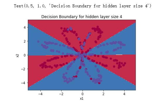
# Print accuracy
predictions = predict(parameters, X)
print ('Accuracy: %d' % float((np.dot(Y, predictions.T) + np.dot(1 - Y, 1 - predictions.T)) / float(Y.size) * 100) + '%')

Output

Accuracy: 90%

Accuracy is really high compared to Logistic Regression. The model has learned the patterns of the flower’s petals! Unlike logistic regression, neural networks are able to learn even highly non-linear decision boundaries.

Congrats on finishing this Programming Assignment!

Here’s a quick recap of all you just accomplished:

• Built a complete 2-class classification neural network with a hidden layer
• Made good use of a non-linear unit
• Computed the cross entropy loss
• Implemented forward and backward propagation
• Seen the impact of varying the hidden layer size, including overfitting.

You’ve created a neural network that can learn patterns! Excellent work. Below, there are some optional exercises to try out some other hidden layer sizes, and other datasets.

6 - Tuning hidden layer size (optional/ungraded exercise)

Run the following code(it may take 1-2 minutes). Then, observe different behaviors of the model for various hidden layer sizes.

# This may take about 2 minutes to run

plt.figure(figsize=(16, 32))
hidden_layer_sizes = [1, 2, 3, 4, 5]

# you can try with different hidden layer sizes
# but make sure before you submit the assignment it is set as "hidden_layer_sizes = [1, 2, 3, 4, 5]"
# hidden_layer_sizes = [1, 2, 3, 4, 5, 20, 50]

for i, n_h in enumerate(hidden_layer_sizes):
    plt.subplot(5, 2, i+1)
    plt.title('Hidden Layer of size %d' % n_h)
    parameters = nn_model(X, Y, n_h, num_iterations = 5000)
    plot_decision_boundary(lambda x: predict(parameters, x.T), X, Y)
    predictions = predict(parameters, X)
    accuracy = float((np.dot(Y,predictions.T) + np.dot(1 - Y, 1 - predictions.T)) / float(Y.size)*100)
    print ("Accuracy for {} hidden units: {} %".format(n_h, accuracy))

Output

Accuracy for 1 hidden units: 67.5 %
Accuracy for 2 hidden units: 67.25 %
Accuracy for 3 hidden units: 90.75 %
Accuracy for 4 hidden units: 90.5 %
Accuracy for 5 hidden units: 91.25 %

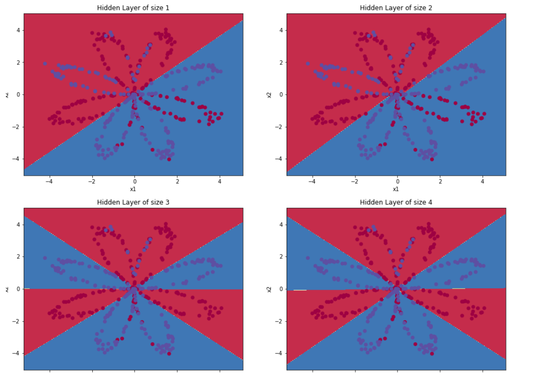
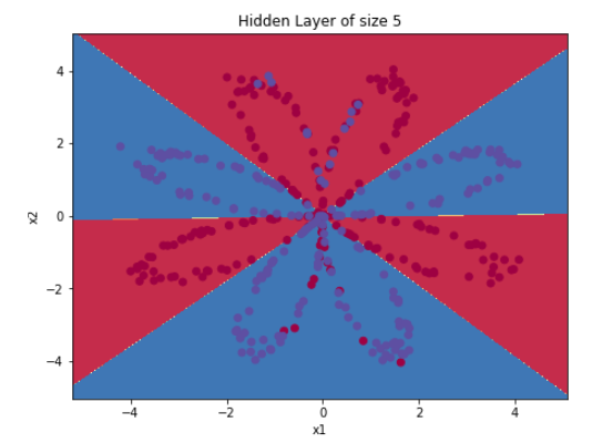
Interpretation:

• The larger models (with more hidden units) are able to fit the training set better, until eventually the largest models overfit the data.
• The best hidden layer size seems to be around n_h = 5. Indeed, a value around here seems to fits the data well without also incurring noticeable overfitting.
• Later, you’ll become familiar with regularization, which lets you use very large models (such as n_h = 50) without much overfitting.

Note: Remember to submit the assignment by clicking the blue “Submit Assignment” button at the upper-right.

Some optional/ungraded questions that you can explore if you wish:

• What happens when you change the tanh activation for a sigmoid activation or a ReLU activation?
• Play with the learning_rate. What happens?
• What if we change the dataset? (See part 7 below!)

7- Performance on other datasets

# Datasets
noisy_circles, noisy_moons, blobs, gaussian_quantiles, no_structure = load_extra_datasets()

datasets = {"noisy_circles": noisy_circles,
            "noisy_moons": noisy_moons,
            "blobs": blobs,
            "gaussian_quantiles": gaussian_quantiles}

### START CODE HERE ### (choose your dataset)
dataset = "noisy_moons"
### END CODE HERE ###

X, Y = datasets[dataset]
X, Y = X.T, Y.reshape(1, Y.shape[0])

# make blobs binary
if dataset == "blobs":
    Y = Y%2

# Visualize the data
plt.scatter(X[0, :], X[1, :], c=Y, s=40, cmap=plt.cm.Spectral);

Output

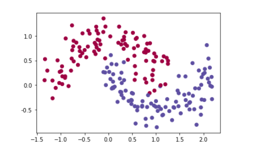
References:

• http://cs231n.github.io/neural-networks-case-study/

Grades

后记

2024年5月11日下午上海下雨。